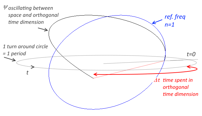
The time dimension present a lower resistance to \(\psi\) and so the time spent, \(\Delta t\) is less than half a period. The frequency of \(\psi\) is thus higher than the reference frequency of \(\psi\) when \(n=1\), but lower than the theoretical frequency when \(n=0.5\).
In fact, since there are three time dimensions, \(t_T\), \(t_g\) and \(t_c\), these correspond to the first three points in the data set repeated below.
| n | \(\lambda\) (nm) | \(\cfrac { n\lambda }{ 2\pi }\) | \(n^{ 2 }ln(\cfrac { 2\pi }{ n\lambda \times10^{-9} } )\) | \(\cfrac { \lambda }{ 2\pi }\) |
|---|---|---|---|---|
| 0.5 | 121.567 | 9.674 | 4.613 | 19.349 |
| 0.5 | 102.573 | 8.162 | 4.656 | 16.325 |
| 0.5 | 97.254 | 7.739 | 4.670 | 15.479 |
Each of this time dimension present different resistance to \(\psi\). The first data corresponds to the highest resistance from the three time dimensions. More \(\Delta t\) spent along that time dimension result in a greater decrease in frequency and a higher corresponding increase in \(\lambda\) compared to half a wavelength.
We have removed the first three data points from the data set, we are left with,
| n | \(f\) |
|---|---|
| 0 | 0 |
| 1 | 3156567.3 |
| 1 | 3196759.8 |
| 1 | 3220973.8 |
| 1 | 3236699.1 |
| 1 | 3247491.0 |
| 1 | 3260914.0 |
| 1 | 3260921.1 |
| 1 | 3265268.4 |
All frequencies are at \(n=1\), ie one wavelength around the perimeter \(2\pi x\). And we are left with just two points on the plot. A theoretical point of \((0,0)\) and one data point.

And so,
\(\cfrac{c}{2\pi a_\psi}=3230699.3\)
\(a_\psi=14.77\) nm
This is the radius of the particle given its spectrum. An electron.
More importantly we might have three other particles oscillating in space and one other time dimension. Each presenting varied resistance against \(\psi\) in the respective time dimension, \(t_T\), \(t_g\) or \(t_c\).