Why Charges Have Mass?

The force \(F_\rho\) to affect a change in \(\psi\) is given by,

\(F_\rho=-\cfrac{\partial\,\psi}{\partial\,x}\)

This force act against the system and results in work done that is equal to a change in energy \(\psi\).  So, the resistance exerted by the system of a solitary particle on an external agent is given by,

\(F_i=-F_\rho=\cfrac{\partial\,\psi}{\partial\,x}\)

where \(F_i\) is the force exerted by the particle on an external agent.  So,

\(F_i=-F_{\rho}=-i\sqrt { 2{ mc^{ 2 } } }\,G.tanh\left( \cfrac { G }{ \sqrt { 2{ mc^{ 2 } } }  } (x-x_z) \right)\)

The following diagram shows the interaction between two monopoles of positive \(F_i\), ie (-\(F_\rho\))

The concentration of \(\psi\) between the two particles pushes them apart.  And their interaction is thus repulsive.

In a similar way, the diagram below shows the interaction between two monopoles of \(-F_i\), ie (+\(F_\rho\))

The depletion of \(\psi\) between the two particles pulls them together.  And their interaction is thus attractive.

Both diagrams show \(F_{\rho}\), the force developed in previous posts, from an external agent affecting a change in \(\psi\) around the particle.  Strictly speaking the force due to the particles are,

And the interaction of two dissimilar particles is,

If the interaction of two positive \(F_i\) is that of charges (repulsive, like charges repel) and the interaction of two \(-F_i\) is that of gravity particle (attractive, two masses attract), then the interaction of \(F_i\) and \(-F_i\) shown above, is attractive as though the charge has mass; the interaction between two masses is attractive.

If the interaction of \(+F_i\) is that of negative charges, then along the negative \(t_c\) time dimension we have positive charges.  Similarly, along \(-t_g\) time dimension, anti-mass particles.

Negative and positive charges are matter/anti-matter pair, and mass and anti-mass are similarly matter/anti-matter pair.

Resistance In Time, Not Futile

What is the resistance to \(\psi\) in space?

\(Z_o=\sqrt{\cfrac{\mu_o}{\varepsilon_o}}\)

this is two dimensional between \(E\) and \(B\) fields. The equivalent of this along one space dimension, assuming that all space dimensions are equivalent is,

\(Z_{1Do}=\cfrac{1}{\sqrt{2}}\sqrt{\cfrac{\mu_o}{\varepsilon_o}}\)

This is the resistance presented by space, encountered by \(\psi\) around a photon, between one time dimension and one space dimension.  Does time exert a resistance to \(\psi\)?  Does it exert the same resistance to \(\psi\) as space?  If it does, then the resistance is the same for a charge as a for a photon, both then will have the same mass and the same extend of \(\psi\) in space.  This is not the case.

So, time and space dimensions are fundamentally different.  The time dimension may exert a resistance to \(\psi\) but this resistance is less than that of space, so much so that a photon manifest fully as energy oscillating between one time and one space dimension. A charge or gravity particle oscillating between two space dimensions has mass and less of an aura of  \(\psi\) around it.

So, \(Z_{1To}\), the resistance to \(\psi\) due to one time dimension is,

\(0\le Z_{1To}\lt \cfrac{1}{\sqrt{2}}\sqrt{\cfrac{\mu_o}{\varepsilon_o}}\)

And the total resistance when \(\psi\) oscillates between one time dimension and one space dimension is,

\(Z_{DTo}=\sqrt{Z^2_{1To}+Z^2_{1Do}}\)

We can now formulate time force, and time energy.

Deforming Photons

So, a mass-less collision with a photon is possible.  During the process the photon gain mass as its \(\psi\) changes to counter the impact.  At the extreme, the photon has the mass of a proton.\(\require{cancel}\)

\(m_{\rho\,ph} c^2=m_{\rho\,po} c^2-\cancelto{0}{\int^{x_a}_{0}{\psi}dx}\)

where \(x_z=0\) and

\(\cfrac{\partial\,F}{\partial\,x}=maximum=-\cfrac{\partial^2\psi}{\partial\,x^2}\)

such that,

\(\Delta F=-\cfrac{\partial^2\psi}{\partial\,x^2}\Delta x\)

At \(x_z=0\), a change in \(\Delta x\) encounters a maximum change in force density.  \(\psi\) deformed and the photon gained mass, but at which point (\(x_z=0\)), a change in \(x\) results in the largest change in \(F\) and the photon readily returns to its original form.  There is no new equilibrium/stable point.

Beam Me Up Scotty!

If there is no constrain on \(x_z\) other than,

\(m_{\rho}c^2-\int^{x_a}_{0}{\psi}dx\ge0\)

since,

\(x_a=2x_z\)

\(m_{\rho}c^2-\int^{2x_z}_{0}{\psi}dx\ge0\)

from the post "We Still Have A Problem", then \(x_z\) can take on all values from

\(0\lt x_z\lt x_{z\,max}\)

where,

\(m_{\rho}c^2=\int^{2x_{z\,max}}_{0}{\psi}dx\)

A particle under no force from its surroundings will tend towards maximum \(\psi\), being mass-less.  Under the action of a force (or to provide a centripetal force) the particle will change its \(\psi\) such that,

\(F=-\cfrac{\partial\,\psi}{\partial\,x}=F_{external}\)

the force \(F\) as a result of \(\psi\) equals the external force as required.

The particle's mass changes as the forces around it.  In the case of a photon oscillating between one time dimension and one space dimension, it experiences less constrain by way of the space dimension than a charge or gravity particle that oscillate between two space dimensions.  So, a photon fully manifest itself as \(\psi\).  A charge or gravity particle experiences more constrain in two dimensions cannot manifest fully as \(\psi\) and so has mass.

If this is true, we can distill a photon to have mass by applying a force in the one space dimension that it is oscillating.  And since a photon can display negative \(\psi\) effects, an electron (charge) or gravity particle can be made mass-less in a stream of photons, where the particle fully manifest itself as \(\psi\).

Under the right conditions we can all turn into pure energy.

Magnetic Monopoles, \(g_B\) Monopoles

The two diagrams below visualize \(F_{\rho}\) from the post "Not Exponential, But Hyperbolic And Positive Gravity!",

\(F_{ \rho  }=i\sqrt { 2{ mc^{ 2 } } } \, G.tanh\left( \cfrac { G }{ \sqrt { 2{ mc^{ 2 } } }  } (x-x_{ z }) \right) \)

The most serious implication is that these are magnetic mono-poles moving in the \(t_c\) time dimension at light speed.  Equivalently, there are  \(g_B\) mono-poles moving in the \(t_g\) time dimension at light speed.

In real time \(t\), we have moving charges generating a \(B\) field perpendicular to the radial line by the right hand screw rule.  The field lines above however, radiate along the radial line.

It could be that as such a particle travels in space, the field lines in space along the path of the particle collapse into a circular path as the particle passes.

There is then no electrostatic force, only the magnetic force.  And there is no gravity but the original force is \(g_B\).

We have a serious problem.  I am floating away already.

Why? Why? Tell Me Why?

From the post "Less Mass But No Theoretical Mass" and "Two Types Of Photons" we have,

\(m_{po}=m\) or equivalently,

\(m_{\rho\,po}=m_{\rho}\)

\(m_{\rho\,e} c^2=m_\rho c^2-\int^{x_a}_{0}{\psi}dx=m_{\rho\,po} c^2-\int^{x_a}_{0}{\psi}dx=m_{\rho\,po} c^2-\int^{2x_z}_{0}{\psi}dx\)

and

\(m_{\rho\,ph} c^2=m_\rho c^2-\int^{x_a}_{0}{\psi}dx=0\)

\(m_\rho c^2=\int^{x_a}_{0}{\psi}dx\)

In general from the post "We Still Have A Probelm",

\(m_{\rho\,particle}c^2+\int^{x_a}_{0}{\psi}dx=m_\rho c^2=m_{\rho\,po} c^2\)

which is of course an assumption that all particles is due to a common manifestation.  In which case, there is one value of \(m_\rho\) and the value of \(x_a=2x_z\), determines what type of particle we have.

\(m_{\rho\,particle}c^2+\int^{2x_z}_{0}{\psi}dx=m_{\rho\,po} c^2\)

Why \(m_{\rho\,po} \) and why \(x_z\)?  Why do these parameters (mass densities, \(m_{\rho\,x}\)), take on the values that they do?

\(m_{\rho\,particle}+\cfrac{1}{c^2}\int^{2x_z}_{0}{\psi}dx=m_{\rho\,po} \)

From symmetry about \(x=x_z\)

\(m_{\rho\,particle}+\cfrac{2}{c^2}\int^{x_z}_{0}{\psi}dx=m_{\rho\,po} \)

When this mass is fully manifested as \(\psi\), we have a photon,

\(E_{\rho\,ph}=\int^{2x_z}_{0}{\psi}dx=m_{\rho\,po} c^2=constant!\)

where \(m_{\rho\,po}\) is the mass density of a proton and \(E_{\rho\,ph}\), the energy density of the photon.

Which, strangely, is consistent with the photons being particles in a helical path, where their kinetic energy is,

\(KE=\cfrac{1}{2}m_{ph}c^2+\cfrac{1}{2}m_{ph}c^2=m_{ph}c^2\)

What happens to photoelectric effects?  \(r\) the radius of the helical path changes inversely with frequency \(f\).

\(2\pi rf=c\),    \(2\pi r=\lambda=\cfrac{c}{f}\)

A smaller \(r\) pushes the electron further towards the nucleus and is ejected with greater velocity after the photon passes.  This means \(r\) is inversely proportional to \(E\), the energy of the ejected electron (from the post "Miss e- Miss e- Not").  And so,

\(E\propto f \)

Still, why \(m_{\rho\,po} \) and why \(x_z\)?  Why do these parameters (mass densities, \(m_{\rho\,x}\)), take on the values that they do?

Photon Collisions, Mass-less Collisions?

From the post "Negative \(\psi\), New Particles, Vampires",  when we have two optical fibers of different refractive index spliced together, the section with higher refractive index will cool down and the section with lower refractive index will heat up when it is carrying a beam of photons.

Only actual experimentation will tell whether a decrease in \(V\), corresponds to an increase or decrease in temperature of the material.

Collisions between material lattice and photons would suggests mass-less collisions that cannot be formulated directly.

夜拂寐 情阑珊
月呼睡 心绪垂
影过檐下灯
时随飞光逝
梦请留 意徘徊
醉枕怀 悠思爱

What is This? Is It Possible?

In the previous post "Particle Collisions", the first example of two types of photons colliding resulted in this possibility with a single velocity swap,

It seems to be a photon that is not at light speed but stationary.  Photons are self propelling dipoles, which means immediately afterwards they are driven towards light speed again.  These particles are then detected as photons with low speed accelerating towards light speed.

Possible.

Particle Collisions

Since particles at light speed cannot accelerate faster, momentum at light speed is then swapped whole between dimensional axes upon collisions.  Collisions can then be viewed as the dimensional axes of the wave breaking up and re-assembled as new particles with multiple pairs of velocity swaps.  The following diagram illustrates two types of photons (postulated) colliding, resulting in the creation of new particles.

After the collision, we have a mechanical wave and a particle postulated in the post "Scintillations In Time", possibly a neutrino.  It is also possible that,

The collision results in a charge being created.  In this case a simultaneous momentum exchange between two pairs of axes, each pair with one axis on each particles, resulted in a photon II and a charge.

Below is another example of particle collision.

In this case, one axis with light speed is paired with another axis on the other colliding particle not at light speed, and their velocity swapped.  Two such velocity swap occurs simultaneously during a single collision.  It would seem that the particle has swap velocity among its axes and rotated. This mechanism is different from where the axes seem to breakup and re-assemble which would require multiple velocity swaps.

However whether such collisions occur under normal circumstances and the result of such collisions being possible is speculative.

The existence of such particles is theoretical, but the way they will collide is certain.

Two Types Of Photons

It seems that an example of such vampire particles is the photon, of which there are two types, charged photons that exist along \(t_c\) dimension but oscillates between \(t_g\) and space, and mass photon that exist along \(t_g\) and oscillates between \(t_c\) and space.

Both types of photons are in light speed in space.

Mass photon transfer energy back and forth \(t_c\) and space, effecting particles on the charge time line.  When a particle receive energy along \(t_c\), it moves forward in time.  When it loses the excess energy it returns.  Given the random motions around the particle, it is likely to be at a different relative location when it returns. A Whacko Jump!

Charged photon transfer energy back and forth \(t_g\) and space.  It would have the same effects as a mass photon but on a mass particle along \(t_g\), not on a charge.

The governing equations are the same as that from when a space dimension has been swapped for a time dimension in the wave equation.  The basic wave equation applicable is,

\(\cfrac{\partial^2\psi}{\partial\,t^2_c}=ic\cfrac{\partial^2\psi}{\partial\,x\partial\,t_c}\)

and

\(\cfrac{\partial^2\psi}{\partial\,t^2_g}=ic\cfrac{\partial^2\psi}{\partial\,x\partial\,t_g}\)

where the time axis has been rotated with a space dimension.  That mean this class of particles travels in space at light space.

Previously, particles of the same wave equation travels along both time axes at light speed, and can be stationary in the space dimensions but still manifest an energy, \(\psi\) around it.

Furthermore, from the post "Less Mass But No Theoretical Mass",

\(m_{\rho\,ph} c^2=m_\rho c^2-\int^{x_a}_{0}{\psi}dx=0\)

\(m_\rho c^2=\int^{x_a}_{0}{\psi}dx\)

but

\(F_{\rho\,ph}=\lim\limits_{m\rightarrow0}i\sqrt { 2{ mc^{ 2 } } }\,G.tanh\left( \cfrac { G }{ \sqrt { 2{ mc^{ 2 } } }  } (x-x_z) \right)=0\)

since photon has no mass.  It is fully manifested as an energy density but does not exert a force field around it.

Time Bias

According to one story on the "The Philadelphia Experiment",  a phase shift of 60^o from the time axis \(t\), results in optical invisibility.  Radar invisibility occurs earlier at 45^o, possibly due to the inability to detect small signal, and noise. Since photons and EMV are charge time, \(t_c\), phenomena, that means shifting by 60^o brings it 90^o to the time axis (\(t_c\)) and so have no effect along \(tc\).

This implies that our existence is actually at \(t^{'}\), 30^o to the vertical, closer to \(t_c\) than \(t_g\).  And when parallel to \(t_g\) because of the phase shift, we should experience the full effects of gravity time; gain mass and feel heavier.

This is wrong. The phase shift also causes the \(t_g\) component of  \(t^{'}\) to be perpendicular to \(t_g\) and so gravity has no effect also.

At the same phase shift, all the electronics/electricals will fail because \(t_c\) is now orthogonal to \(t^{'}\).

Scintillations In Time

This is another possible particle, where energy oscillates between two time dimensions (\(t_c\) and \(t_g\)) and it travels down two space dimensions at light speed.  We have seen how such motion is possible when the particle travels in a helical path.  However, since such particle oscillates on the time axes, it is not with us in time (we travel on the time axis at light speed), but fade into existence and then fade out of existence.

Its mass which is equivalent to its kinetic energy along the time axis \(t_g\) oscillates as the particle oscillates.  It has a charge but such a charge (which is the analogue of mass on the time \(t_c\) axis) oscillates as the particle oscillates.

Such particles will be difficult to detect as they scintillate in and out of existence.  A neutrino, maybe.

Negative \(\psi\), New Particles, Vampires

If \(\psi\) is negative and all energy is equivalent to kinetic energy along a time dimension ("Precession Under Zero Gravity"),

\(\int^{x}_{0}{\psi}\,dx=-m_{\rho}c^2\)

then,

\(\int^{x}_{0}{\psi}\,dx=m_{\rho}(ic)^2\)

this is possible in a wave where energy oscillates between two orthogonal dimensions, here denoted by,

\(c\) and \(ic\)

Energy oscillations between two space dimensions will not manifest negative \(\psi\) as the total \(\psi\) across both space dimensions, both accessible in our reality, sum to a positive constant.

If energy oscillations are between two time dimensions, a third time dimension is then necessary for the phenomenon to exist, by which all time based calculation are made.

If energy oscillations are between one time dimensions and one space dimension, energy drain from the space dimension will be seen as negative energy as the total energy in 3D space will decrease.  This kind of particle will require another time dimension on which to exist and be at light speed, and another space dimension on which it is also at light speed so that particle is a wave.

This particle will take away energy without itself gaining energy (in space).  The gained energy is in the time dimension, that is part of a space-time dimensional pair between which energy oscillates.  Since it is energy oscillations, the particle can also give energy without itself losing energy.

Both \(t_c\) and \(t_g\) are possible candidates for the space-time dimensional pair; all three space dimensions are also available. This makes two types of such particles as the space dimensions are all equivalent,

\(m_{vc}\) and \(m_{vg}\)

that exist on the \(t_c\) time dimension and \(t_g\) time dimension respectively.  And \(v\) is for Vampire.

\(m_{vc}\) is charged and has energy oscillating between \(t_g\) and a space dimension.  \(m_{vg}\) is not charged and has energy oscillating between \(t_c\) and a space dimension.

How then to detect such particles?  These particles require light speed in space to manifest as a wave, ie \(\dot{x}=c\), which is the difference between them and the particles responsible for charge and gravity.    From the post "My Own Wave Equation",

\(\left(1+\cfrac{1}{\gamma^2} \right)\cfrac { \partial \, \psi  }{ \partial \, t_{ c } }=2\cfrac { \partial V\,  }{ \partial \, t_{ c } }\)

where,

\(\cfrac{1}{\gamma^2}=\left( 1-\cfrac { \dot { x } ^{ 2 } }{ c^{ 2 } }  \right)\)

As \(T\) and \(V\) are symmetrical,  because \(\psi=T+V\).  Given, \(\dot{x}=c\),

\(\cfrac { \partial \, \psi  }{ \partial \, t_{ c } }=2\cfrac { \partial V\,  }{ \partial \, t_{ c } }\)

if however, the particle is to slow down \(\dot{x}\lt c\), then

\(\cfrac { \partial \, \psi  }{ \partial \, t_{ c } }=\cfrac{2}{\left(1+\cfrac{1}{\gamma^2} \right)}\cfrac { \partial V\,  }{ \partial \, t_{ c } }\)

which casues

\(\cfrac { \partial V\,  }{ \partial \, t_{ c } }\) to increase.

If \(V\) is energy in the time dimension, there will be a

decrease in \(\cfrac { \partial T\,  }{ \partial \, t_{ c } }\)

in the space dimension.

because \(\cfrac { \partial \, \psi  }{ \partial \, t_{ c } }=\cfrac { \partial T\,  }{ \partial \, t_{ c } }+\cfrac { \partial V\,  }{ \partial \, t_{ c } }\)

This results in a shift of energy to \(V\) and energy perceived only in space, \(T\) decreases.  In other words, the particle cools.  The space, denoted by \(x_2\) here, as the particle passes however, cools down.  The gain in \(V\) is in the time dimension.  The total \(\psi\) however remains a constant, this shift in \(V\) corresponds to a shift in the center of oscillation.

If the particle has a lower velocity to start with (ie. \(\dot{x}\lt c\)) and then is accelerated to \(c\), a decrease in \(V\) will shift the center of oscillation toward \(T\); \(T\) increases.  If these changes in velocity of the particles happen across two materials, then we have an energy pump that transfer energy from one material to another.

Have a nice day.

Afternote:

Cooling photons will be oscillating between \(t_T\), the thermal time dimension and one other space dimension.  Please refer to later posts on \(t_T\), starting with "3 Space, 3 Time Dimensions And Sesame Street".

Less Mass But No Theoretical Mass

The diagram below shows the case when \(x_z\) is small,

For \(\psi\) to exist, \(F\) is negative for values of \(x\lt x_z\), this would imply that when two positive charges are brought very close together they would attract each other and stick.

Otherwise the mass of a positive is just the mass of the particle along time \(t_c\) when \(x_z=0\),

\(m_{po}=m\)

and

\(m_{\rho\,e} c^2=m_\rho c^2-\int^{x_a}_{0}{\psi}dx=m_{\rho\,po} c^2-\int^{x_a}_{0}{\psi}dx=m_{\rho\,po} c^2-\int^{2x_z}_{0}{\psi}dx\)

In both cases,

\(m_{\rho\,e}\lt m_{\rho\,po} \)

because

\(x_{z\,po}\lt x_{z\,e}\)

that more of the \(F\) curve associated with a negative charge is negative, than the \(F\) curve associated with a positive charge.

We Still Have A Problem

A diagram of the time axes \(t_c\) and \(t_g\) is shown below,

and from the post "Not Exponential, But Hyperbolic And Positive Gravity!",

\(\int { 1 } d\, x=-i2{ mc^{ 2 } }\int { \cfrac { 1 }{ F^{ 2 }-A }  } dF\)

\(x=i2{ mc^{ 2 } }\cfrac { 1 }{ \sqrt { A }  } archtanh(\cfrac { F }{ \sqrt { A }  } )+x_z\)

why would \(x_z\) take on different values of opposite sign?

A plot of log(cosh(x)) with \(x_z=0\) is shown below,

For the case of \(x_z\le0\), \(\psi\lt 0\) for \(x\gt 0\), and \(\int^x_{0}{\psi}dx\rightarrow-\infty\) as \(x\rightarrow \infty\), this would require infinite negative energy to realize.  So \(x_z \gt 0\), and \(0\lt x\le x_a\), where at \(x=x_a\), \(\psi=0\) such that \(\int^{x_a}_{0}{\psi}dx=+finite\) and so does not require infinite amount of energy.

If this is the case than,

A more negative value in \(F\) appears as \(x_z\) increases and

\(\int^{x_a}_{0}{\psi}dx\), the total \(\psi\) over the extend of \(x_a\) increases.  Could it be that,

\(m_{\rho\,particle} c^2=m_\rho c^2-\int^{x_a}_{0}{\psi}dx\)

that the energy, \(m_{\rho\,particle}c^2\) associated with the mass density of the particle, \(m_{\rho\,particle}\) in real time is the result of the total \(\psi\) being subtracted from the total kinetic energy, \(m_\rho c^2\) along the \(t_c\) (or \(t_g\)) dimension.  This reduction in mass density is  to provide for the total \(\psi\).  Such that when the particle is annihilated the total amount of energy released is,

\(m_{\rho\,particle}c^2+\int^{x_a}_{0}{\psi}dx=m_\rho c^2\)   (per unit volume)

where \(m_\rho\) is the mass density of the particle along time \(t_c\) (or \(t_g\)), and \(m_{\rho\,particle}\) is the mass density of the particle in \(t\) time dimension.

This means, when a particle is a wave in two space dimensions and one time dimension, together with a fourth time dimension along which it exists, part of its mass \(m\), is fuzzed into an energy density field in 3D space and real time \(t\) around the particle.  The remaining energy manifest its self as \(m_{p}\), the mass of the particle in 3D space and real time \(t\).

This is the reason why an electron has lower mass, part of its mass is manifested as \(\psi\) around it.

What then is this value of \(m\) to start with?  If \(m_{\rho}\) is a positive value, that means the constrain on \(x_a\) is,

\(m_{\rho}c^2-\int^{x_a}_{0}{\psi}dx\ge0\)

ie. as long as \(m_{\rho\,particle}\ge0\).  And given that \(F\) has rotational symmetry about the origin,

\(F(x)=-F(-x)\),

\(x_a=2x_z\)

We have one constrain on the value of \(x_z\).

This however does not restrict the values of \(x_z\) and the corresponding \(x_a=2x_z\) for specifically an electron or the analogous gravity particle.

Something Old, Something New, A Shoulder To Rely On

From the post "We Have A Problem, Coulomb's Law",

\(F=2\cfrac { mc^{ 2 } }{ x } e^{i\pi/2}\)

So,

\(\psi=-\int{2\cfrac { mc^{ 2 } }{ x } e^{i\pi/2}}d\,x\)

\(\psi=-{2{ mc^{ 2 } }{ ln(x) } e^{i\pi/2}}\)

Similarly \(\psi\) is delimited at \(x=x_a\), where \(\psi=0\).  However, without \(A\) (cf. post "Not Exponential, But Hyperbolic And Positive Gravity!"), Coulomb's Law applies for all \(x\gt0\).

\(F=\cfrac { mc^{ 2 } }{ 6\pi x^2 } e^{i\pi/2}\)

Nice to know there's something old to fall back on.

The Truth Of Two Strong Magnets

Two strong magnets set to attract each other (N,S poles facing each other), brought from a distance apart, pushes each other sideways first then on closer proximity attract each other.

I have always wondered why attracting magnets go sideways but I can move them to be perfectly aligned after they are stuck together.

Have a nice day.

Not Quite The Same Newtonian Field

From the post "Not Exponential, But Hyperbolic And Positive Gravity!", the force density associated with \(\psi\) around a stationary particle is,

\(F_{\rho}=i\sqrt { 2{ mc^{ 2 } } }\,G.tanh\left( \cfrac { G }{ \sqrt { 2{ mc^{ 2 } } }  } (x-x_z) \right)\)

and so the energy density, is given by,

\(-\cfrac{\partial\,\psi}{\partial\,x}=F_{\rho}\)

\(\psi=-\int{i\sqrt { 2{ mc^{ 2 } } }\,Gtanh\left( \cfrac { G }{ \sqrt { 2{ mc^{ 2 } } }  } (x-x_z) \right)}dx\)

\(\psi=-i{ 2{ mc^{ 2 } } }\,ln(cosh(\cfrac { G }{ \sqrt { 2{ mc^{ 2 } } }  }(x-x_z)))+c\)

when \(x=0\), \(\psi=0\)

\(c=i{ 2{ mc^{ 2 } } }\,ln(cosh(\cfrac { G }{ \sqrt { 2{ mc^{ 2 } } }  }x_z))\)

A plot of tanh(x-1) and -log(cos(x-1)) is given below,

 \(x=x_a\) where \(\psi=0\) delimits the physical extend of \(\psi\) as we consider only positive energy, \(\psi\) cannot be negative.  The plot is illustrative only, the value of \(x_a\) is scale by the factor,

\(\cfrac { G }{ \sqrt { 2{ mc^{ 2 } } }  }\)

\(F_{\rho}\) is valid up to when \(\psi=0\) at \(x=x_a\).  Since,

 \(\psi(x)=\psi(-x)\) and \(\psi\) is symmetrical about the \(y=0\) axis.

The shape of \(\psi\) depends on \(x_z\).  In this case, it is a double bell centered at \(x\) with \(x_z=1\)

The 3D plot is generated using scilab

  o=0.0;

    for n=1:(1/0.02)

        t = 0:0.01:(2.0*%pi);

        x=o*ones(1,size(t,'c'));

        r=-(log(cosh(o-0.5))-(log(cosh(-0.5))));

        y = r*sin(t);

        z = r*cos(t);

        param3d(x,y,z,45,60,"X@Y@Z",[2,3]);

        o=o+0.02;

    end

    o=0.0;

    for n=1:(1/0.02)

        t = 0:0.01:(2.0*%pi);

        x=-1*o*ones(1,size(t,'c'));

        r=-(log(cosh(o-0.5))-(log(cosh(-0.5))));

        y = r*sin(t);

        z = r*cos(t);

        param3d(x,y,z,45,60,"X@Y@Z",[2,3]);

        o=o+0.02;

    end

Two collapsed views are also plotted,

collapsed along the y-axis.

collapsed along the x-axis, the plot is a perfect circle.  A plot corresponding to a smaller value of \(x_z=0.5\) is also given,

Except for smaller average radius, it is essentially the same shape as the previous plots.  These are plots of energy density along the \(\pm\) x-axis of a single particle.  These are not electron clouds in 3D.  If we plot the contour of maximum \(\psi\) around the particle, it is just a sphere.

There is a problem, \(F_{\rho}\) beyond \(x_a\) is zero.  In the old formulation of gravity or electrostatic force, \(F\rightarrow0\) as \(x\rightarrow\infty\), the associated field stretches to infinity, and does not abruptly decrease to zero.  In the case of gravity, not only does the field density drop to zero abruptly, it is positive, pushing mass outwards just before disappearing.

The fact is \(F_{\rho}\) is not \(F\).  At \(x=x_a\),

\(F_{\rho}(x_a)=F_{xa}\)

For \(x\gt x_a\),

\(F=F_{xa}\cfrac{4}{3}\pi x^3_a\cfrac{1}{4\pi x^2_a}\cfrac{1}{4\pi x^2}=\cfrac{1}{12\pi x^2}F_{xa}x_a\)

where \(F_{xa}\) is a constant.  This formula is valid for \(x\ge x_a\) and since both \(F_{xa}\) and \(x_a\) are constants, it obeys Coulomb's Law.

So, the force field around a particle can be divided in two, a near field \(x\lt x_z\) and a far field \(x\ge x_a\).

Detecting Electrons With Electrons

What does,

\(\cfrac { \partial ^{ 2 }\, \psi  }{ \partial \, t^{ 2 }_{ c } } =(ic)^{ 2 }\cfrac { \partial ^{ 2 }\, \psi  }{ \partial \, x^{ 2 } } =-c^{ 2 }\cfrac { \partial ^{ 2 }\, \psi  }{ \partial \, x^{ 2 } }\)

mean to be a wave in time dimension \(t_c\)?  Simply, that it has to be detected in the time \(t_c\) dimension.  All that is needed is an electric/electronic device.  In the \(t_g\) time dimension it is not detected, an weighing machine will not be able to detect the wave, not directly.

Shifty Tanh(x) And Consistency

From the posts "Not Exponential, But Hyperbolic And Positive Gravity!" and "Flux It", \(F\) due to the particles travelling as a wave in two time dimensions (\(t_g\) and \(t_c\)) and one space dimension that manifest the field phenomenon without the particle moving in space in our 3D space/time \(t\) dimension,

\(F=i\cfrac{\sqrt { 2{ mc^{ 2 } } }}{12\pi x}\,G.tanh\left( \cfrac { G }{ \sqrt { 2{ mc^{ 2 } } }  } (x-x_z) \right)\)

=================================================================
Note 26 May 2015:  This equation is wrong.  Please refer to post "Opps! Lucky Me" and "Wrong, Wrong Wrong" both dated 25 May 2015.  Instead,

\(F=\int{F_\rho}\,d\,x\)

=================================================================
where \(x_z\) is the constant of integration after a second and last integration, the specific value of \(x_z\) can account for why particles in the same direction along the \(t_g\) time axis attract each other but particles in the same direction along the \(t_c\) time axis repel each other.  Plots of \(F\) with \(x_z=0\), \(x_z=-1\) and \(x_z=+1\) is shown below,

A positive \(x_z\) results in a attractive force such as gravity and a negative \(x_z\) results in a repulsive force that does not cross into the negative values of \(F\).  A zoomed view of the two types of forces are plotted below

Now we have a consistent view for both gravity and the electrostatic force.  Except for the fact that, the attractive force turns repulsive before its approach to zero as \(x\rightarrow\infty\), which needs further verification.

With the new wave equation from the post "My Own Wave Equation",

\(\ddot { x } \left( 2-i\cfrac { \dot { x }  }{ c }  \right) \cfrac { \partial \, \psi  }{ \partial \, t_{ c } } =ic\left( 1+i\cfrac { \dot { x }  }{ c }  \right) \dot { x } ^{ 2 }\cfrac { \partial ^{ 2 }\psi  }{ \partial \, x^{ 2 } } +2\ddot { x } \cfrac { \partial V\,  }{ \partial \, t_{ c } }\)

we also have MY VERY OWN UNIFIED THEORY!

Flux It,

The derivation for force in this post is wrong, although the conclusion that the force is zero at infinity is true.  Please refer to posts "Opps! Lucky Me" and "Flux It Too" dated 25 May 2015.

The following diagram shows the force density, \(F_\rho\), on the surface of a sphere at a radius \(x\),

The total force within the volume, \(F_v\) is,

\(F_{ v }=F_{ \rho  }\cfrac { 4 }{ 3 } \pi \, x^{ 3 }\)

Imagine all this forces being distributed uniformly on the surface of the sphere (\(4\pi x^2\)), the total flux is then,

\(F_{ A }=F_{ \rho  }\cfrac { 4 }{ 3 } \pi \, x^{ 3 }\cfrac { 1 }{ 4\pi \, x^{ 2 } } \)

When the total flux is conserved, at \(x_1\) and \(x_2\)

\(F_{ 1 }.4\pi \, x^{ 2 }_{ 1 }=F_{ 2 }.4\pi \, x^{ 2 }_{ 2 }=F_{ A }\)

\(F_{ 1 }=F_{ A }\cfrac{1}{4\pi \, x^{ 2 }_{ 1 }}\)

as such given a general radial distance \(x\),

\(F=\cfrac { F_{ A } }{ 4\pi \, x^{ 2 } } =F_{ \rho  }\cfrac { 4 }{ 3 } \pi \, x^{ 3 }\cfrac { 1 }{ 4\pi \, x^{ 2 } } \cfrac { 1 }{ 4\pi \, x^{ 2 } } =F_{\rho}\cfrac{1}{12\pi x}\)

\(F\), \(F_1\) and \(F_2\) are in Newtons (N).

So, if the force density, \(F_{\rho}\) is a constant as in the post "Constant Of Integration Used Up", then

\(F=F_{\rho}\cfrac{1}{12\pi x}\),  \(F_{\rho}=constant\)

\(F\rightarrow 0\), as \(x\rightarrow\infty\)

It is not absurd after all.  And the universe is safe from ever expanding.

\(F=i\cfrac{\sqrt { 2{ mc^{ 2 } } }}{12\pi x}\,G.tanh\left( \cfrac { G }{ \sqrt { 2{ mc^{ 2 } } }  } (x-x_z) \right)\)

There is no need for \(g_o\) to shift \(-F\) up.

It is however still very interesting that \(F\) should reverse sign, and turn positive.

A comparative plots of \(\cfrac{1}{x^2}\), \(\cfrac{1}{x}tanh(x-1)\)  and \(\cfrac{1}{x}\) is given above.  \(tanh(x)\) is the lowest of them all, and passes below \(y=0\) before tending towards zero as \(x\rightarrow\infty\).

This positive gravity outwards might explain why some asteroid (unconfirmed report of 2012 da14 asteroid is slowing down) decelerate on approach to earth.

Constant Of Integration Used Up

If we consider \(F\) from the previosu post "Not Exponential, But Hyperbolic And Positive Gravity!" further,

\(F=i\sqrt { 2{ mc^{ 2 } } }\,G.tanh\left( \cfrac { G }{ \sqrt { 2{ mc^{ 2 } } }  } (x-x_z) \right)\)

when \(x_z\) is large, a plateau value for \(-F\) emerged as illustrated below.

The absurd point is that as \(x\rightarrow\infty\), \(g=constant\).  If \(-F\) is shifted upwards by \(g_o\) such that,

\(F=i\sqrt { 2{ mc^{ 2 } } }\,G.tanh\left( \cfrac { G }{ \sqrt { 2{ mc^{ 2 } } }  } (x-x_z) \right)+g_o\)

where,

\(g_o=i\sqrt { 2{ mc^{ 2 } } }\,G.tanh\left( \cfrac { G }{ \sqrt { 2{ mc^{ 2 } } }  } (-x_z) \right)\)

\(g_o=-i\sqrt { 2{ mc^{ 2 } } }\,G.tanh\left( \cfrac { G }{ \sqrt { 2{ mc^{ 2 } } }  } x_z \right)\)

and \(F\rightarrow 0\)  as  \(x\rightarrow\infty\).

But what would be the rationale to do so??

However, this absurdity does provide a constant force that propels the mass particle to light speed, \(\dot{x}=c\), which was one of the possible scenario considered previously.

Not Exponential, But Hyperbolic And Positive Gravity!

From the post "We Have A Problem, Coulomb's Law", we formulated the expression for \(F\),

\(\cfrac{F}{m}\cfrac { \partial ^{ 2 }\, \psi  }{ \partial \, x^{ 2 } } =-i c^{ 2 } (\cfrac { \partial ^{ 2 }F }{ \partial \, x^{ 2 } } )\)

but  \( \cfrac { \partial ^{ 2 }\, \psi  }{ \partial \, x^{ 2 } } =\cfrac { \partial F }{ \partial \, x } \)

So,

\(F\cfrac { \partial \, F }{ \partial \, x } =-i mc^{ 2 } (\cfrac { \partial ^{ 2 }F }{ \partial \, x^{ 2 } } )\)

\( \cfrac { 1 }{ 2 } \cfrac { \partial \, F^{ 2 } }{ \partial \, x } =-imc^{ 2 }(\cfrac { \partial ^{ 2 }\, F }{ \partial \, x^{ 2 } } )\) --- (*)

If we consider a constant term after the first integration,

\(F^{ 2 }-A=-i2{ mc^{ 2 } }\cfrac { \partial F }{ \partial \, x } \)

This term corresponds to loss in \(F\) as it progresses along \(x\).  This is equivalent to \(F\) being in a medium with mass, ie. space has inertia.

\( \int { 1 } d\, x=-i2{ mc^{ 2 } }\int { \cfrac { 1 }{ F^{ 2 }-A }  } dF\)

\(x=i2{ mc^{ 2 } }\cfrac { 1 }{ \sqrt { A }  } archtanh(\cfrac { F }{ \sqrt { A }  } )+x_z\)

\(-i\cfrac { \sqrt { A } (x-x_z) }{ 2{ mc^{ 2 } } } =archtanh(\cfrac { F }{ \sqrt { A }  } )\)

\(F=\sqrt { A } tanh\left( \cfrac { {- i\sqrt { A }  } }{ 2mc^{ 2 } }( x-x_z) \right) \)

From (*) it is possible that

\(F^{ 2 }=-2i{ mc^{ 2 } }\left(\cfrac { \partial F }{ \partial \, x }+D^2\right) \)

where \(D^2\) is the constant of integration,

\(F^{ 2 }+i2{ mc^{ 2 }D^2 }=-i2{ mc^{ 2 } }\cfrac { \partial F }{ \partial \, x } \)

and so,

\( A=-i2{ mc^{ 2 } }D^2=e^{i3\pi/2}.2{ mc^{ 2 } }D^2\),

\( \sqrt{A}=e^{i3\pi/4}D\sqrt{2{ mc^{ 2 }}}\),

\(-i\sqrt{A}=e^{-i\pi/2}.e^{i3\pi/4}D\sqrt{2{ mc^{ 2 }}}=e^{i\pi/4}D\sqrt{2{ mc^{ 2 }}}\)

Therefore,

\(F=e^{ i3\pi /4 }D\sqrt { 2{ mc^{ 2 } } } .tanh\left( \cfrac { { D } }{ \sqrt { 2{ mc^{ 2 } } }  }( x-x_o).e^{ i\pi /4 } \right) \)

If \(G=D.e^{ i\pi /4 }\) is real then

\(F=e^{i\pi/2}\sqrt { 2{ mc^{ 2 } } }\,G.tanh\left( \cfrac { G }{ \sqrt { 2{ mc^{ 2 } } }  } (x-x_z) \right) \)

\(F=i\sqrt { 2{ mc^{ 2 } } }\,G.tanh\left( \cfrac { G }{ \sqrt { 2{ mc^{ 2 } } }  } (x-x_z) \right) \)

where \(e^{i\pi/2}=i\) is interpreted as a phase lag in time. An illustrative plot of \(-F\), which is often the case where minus gravity, \(-g\) is shown,

This solution suggests that there is a zero gravity value in the space around a body at some point \(x_z\), beyond this point gravity is positive and pushes other mass away.

The series expansion of \(\tanh(x)\) is given by,

\(tanh(x)=x-\frac { 1 }{ 2 } x^{ 3 }+\frac { 2 }{ 15 } x^{ 5 }-\frac { 17 }{ 315 } x^{ 7 }...\left| x \right| \)

\(tanh(x)\approx x\).  This is a different result from when \(A=0\).

This force, \(F\) was derived from energy density, as such it is a force per unit volume, ie Nm^-3.  To obtain the normal Newtonian formulation, \(F_g\),

\(F_g(x)=F\cfrac{4}{3}\pi x^3\cfrac{1}{4\pi x^2}\cfrac{1}{4\pi x^2}=F\cfrac{1}{12\pi x}\)

Note: \(arctan\left( x \right) =i\frac { 1 }{ 2 } ln\left( \cfrac { 1-ix }{ 1+ix }  \right) \)

My Own Wave Equation

From the post "Not A Wave But Work Done!",

\(\ddot { x } \left( 2-i\cfrac { \dot { x }  }{ c }  \right) \cfrac { \partial \, \psi  }{ \partial \, t_{ c } } =ic\left( 1+i\cfrac { \dot { x }  }{ c }  \right) \dot { x } ^{ 2 }\cfrac { \partial ^{ 2 }\psi  }{ \partial \, x^{ 2 } } +2\ddot { x } \cfrac { \partial V\,  }{ \partial \, t_{ c } }\) --- (*)

derived under the assumption that \(\dddot{x}=0\), a time invariant field.

Multiply (*) by \(i\),

 \(i\ddot { x } \left( 2-i\cfrac { \dot { x }  }{ c }  \right) \cfrac { \partial \, \psi  }{ \partial \, t_{ c } } =-c\left( 1+i\cfrac { \dot { x }  }{ c }  \right) \dot { x } ^{ 2 }\cfrac { \partial ^{ 2 }\psi  }{ \partial \, x^{ 2 } } +2i\ddot { x } \cfrac { \partial V\,  }{ \partial \, t_{ c } } \)

Multiply by \(\left( 1-i\cfrac { \dot { x }  }{ c }  \right) \),

\( i\ddot { x } \left( 2-i\cfrac { \dot { x }  }{ c }  \right) \left( 1-i\cfrac { \dot { x }  }{ c }  \right) \cfrac { \partial \, \psi  }{ \partial \, t_{ c } } =-c\left( 1-\cfrac { \dot { x } ^{ 2 } }{ c^{ 2 } }  \right) \dot { x } ^{ 2 }\cfrac { \partial ^{ 2 }\psi  }{ \partial \, x^{ 2 } } +2i\left( 1-i\cfrac { \dot { x }  }{ c }  \right) \ddot { x } \cfrac { \partial V\,  }{ \partial \, t_{ c } } \)

\( c\left( 1-\cfrac { \dot { x } ^{ 2 } }{ c^{ 2 } }  \right) \dot { x } ^{ 2 }\cfrac { \partial ^{ 2 }\psi  }{ \partial \, x^{ 2 } } =-i\ddot { x } \left( 2-\cfrac { \dot { x } ^{ 2 } }{ c^{ 2 } } -3i\cfrac { \dot { x }  }{ c }  \right) \cfrac { \partial \, \psi  }{ \partial \, t_{ c } } +2\left( \cfrac { \dot { x }  }{ c } +i \right) \ddot { x } \cfrac { \partial V\,  }{ \partial \, t_{ c } } \)

\( c\left( 1-\cfrac { \dot { x } ^{ 2 } }{ c^{ 2 } }  \right) \dot { x } ^{ 2 }\cfrac { \partial ^{ 2 }\psi  }{ \partial \, x^{ 2 } } =-\ddot { x } \left\{3\cfrac { \dot { x }  }{ c } +i(2-\cfrac { \dot { x } ^{ 2 } }{ c^{ 2 } } ) \right\} \cfrac { \partial \, \psi  }{ \partial \, t_{ c } } +2\left( \cfrac { \dot { x }  }{ c } +i \right) \ddot { x } \cfrac { \partial V\,  }{ \partial \, t_{ c } } \)

Equating Real terms,

\( c\left( 1-\cfrac { \dot { x } ^{ 2 } }{ c^{ 2 } }  \right) \dot { x } ^{ 2 }\cfrac { \partial ^{ 2 }\psi  }{ \partial \, x^{ 2 } } =-3\cfrac { \dot { x }  }{ c } \ddot { x } \cfrac { \partial \, \psi  }{ \partial \, t_{ c } } +2\cfrac { \dot { x }  }{ c } \ddot { x } \cfrac { \partial V\,  }{ \partial \, t_{ c } } \)

\( c\left( 1-\cfrac { \dot { x } ^{ 2 } }{ c^{ 2 } }  \right) \dot { x } \cfrac { \partial ^{ 2 }\psi  }{ \partial \, x^{ 2 } } =\cfrac { \ddot { x }  }{ c } \left\{-3\cfrac { \partial \, \psi  }{ \partial \, t_{ c } } +2\cfrac { \partial V\,  }{ \partial \, t_{ c } }  \right\} \)

Let's define

\(\cfrac{1}{\gamma^2}=\left( 1-\cfrac { \dot { x } ^{ 2 } }{ c^{ 2 } }  \right) \)

We have,

\( \cfrac{c^2}{\gamma^2} \dot { x } \cfrac { \partial ^{ 2 }\psi  }{ \partial \, x^{ 2 } } ={ \ddot { x }  } \left\{- 3\cfrac { \partial \, \psi  }{ \partial \, t_{ c } } +2\cfrac { \partial V\,  }{ \partial \, t_{ c } }  \right\} \) --- (**)

Equating Imaginary terms,

\( -\ddot { x } (2-\cfrac { \dot { x } ^{ 2 } }{ c^{ 2 } } )\cfrac { \partial \, \psi  }{ \partial \, t_{ c } } +2\ddot { x } \cfrac { \partial V\,  }{ \partial \, t_{ c } } =0\)

\(\ddot{x}\ne 0\)

\( (2-\cfrac { \dot { x } ^{ 2 } }{ c^{ 2 } } )\cfrac { \partial \, \psi  }{ \partial \, t_{ c } }=2\cfrac { \partial V\,  }{ \partial \, t_{ c } } \)

\(\cfrac { \partial \, \psi  }{ \partial \, t_{ c } } +\left( 1-\cfrac { \dot { x } ^{ 2 } }{ c^{ 2 } }  \right) \cfrac { \partial \, \psi  }{ \partial \, t_{ c } }=2\cfrac { \partial V\,  }{ \partial \, t_{ c } }  \)

\(\left(1+\cfrac{1}{\gamma^2} \right)\cfrac { \partial \, \psi  }{ \partial \, t_{ c } }=2\cfrac { \partial V\,  }{ \partial \, t_{ c } }\) --- (***)

Substitute the above into (**),

\(\cfrac { c^{ 2 } }{ \gamma ^{ 2 } } \dot { x } \cfrac { \partial ^{ 2 }\psi  }{ \partial \, x^{ 2 } } =-{ \ddot { x }  }\left\{ 3\cfrac { \partial \, \psi  }{ \partial \, t_{ c } } -\left( 1+\cfrac { 1 }{ \gamma ^{ 2 } }  \right) \cfrac { \partial \, \psi  }{ \partial \, t_{ c } }  \right\} \)

\( \cfrac { c^{ 2 } }{ \gamma ^{ 2 } } \dot { x } \cfrac { \partial ^{ 2 }\psi  }{ \partial \, x^{ 2 } } =-{ \ddot { x }  }\left\{ 2-\cfrac { 1 }{ \gamma ^{ 2 } }  \right\} \cfrac { \partial \, \psi  }{ \partial \, t_{ c } }\) --- (1)

\({ \ddot { x }  }\cfrac { \partial \, \psi  }{ \partial \, t_{ c } } =-\cfrac { c^{ 2 } }{ \left\{ 2\gamma ^{ 2 }-1 \right\}  } \dot { x } \cfrac { \partial ^{ 2 }\psi  }{ \partial \, x^{ 2 } } \)

Equivalently from (1),

\({\left( 1+\cfrac { \dot { x } ^{ 2 } }{ c^{ 2 } }  \right) \ddot { x }  } \cfrac { \partial \, \psi  }{ \partial \, t_{ c } } =-c^{ 2 }\left( 1-\cfrac { \dot { x } ^{ 2 } }{ c^{ 2 } }  \right) \dot { x } \cfrac { \partial ^{ 2 }\psi  }{ \partial \, x^{ 2 } } \)

This suggests that when \(\dot{x}=c\), \(\cfrac{1}{\gamma^2}=0\)

\({ 2\ddot { x }  }\cfrac { \partial \, \psi  }{ \partial \, t_{ c } }=0\)

Then either,

 \(\ddot{x}=0\) and \( \cfrac { \partial \, \psi  }{ \partial \, t_{ c } }= \cfrac { \partial \, V }{ \partial \, t_{ c } }\)

or,

\(\cfrac { \partial \, \psi  }{ \partial \, t_{ c } }=0\),

that the total energy of the system is a constant in time \(t_c\) and is at an extrema.  In this case \(\psi\) has a stable point when \(\dot{x}=c\).  From (***),

\(\cfrac { \partial \psi  }{ \partial \, t_{ c } }=2\cfrac { \partial V\,  }{ \partial \, t_{ c } }=0\)

when \(\dot{x}=c\), and

\(\cfrac { \partial^2 \psi  }{ \partial \, t^2_{ c } }=2\cfrac { \partial^2 V\,  }{ \partial \, t_{ c }^2 }\)

\(\psi\) is minimum when \(V\) is at its local maximum.  This shows that the system, as far as \(\psi\), the total energy is concerned, can be stable at light speed, \(\dot{x}=c\).  At that point \(V\) is at its local maximum.

We now consider the case when \(\dot{x}\lt\lt c\),

\({ \ddot { x }  } \cfrac { \partial \, \psi  }{ \partial \, t_{ c } } =-c^{ 2 } \dot { x } \cfrac { \partial ^{ 2 }\psi  }{ \partial \, x^{ 2 } } \)

\({m \ddot { x }  } \cfrac { \partial \, \psi  }{ \partial \, t_{ c } } =-c^{ 2 }m \dot { x } \cfrac { \partial ^{ 2 }\psi  }{ \partial \, x^{ 2 } } \)

With \(F=m\ddot{x}\)  and \(p=m\dot{x}\),

\(F\cfrac { \partial \, \psi  }{ \partial \, t_{ c } } =-c^{ 2 }p \cfrac { \partial ^{ 2 }\psi  }{ \partial \, x^{ 2 } } \)

Since, \(-\cfrac { \partial \, \psi  }{ \partial x } =F=m\ddot { x } \)

\(\cfrac { \partial \, \psi  }{ \partial x } \cfrac { \partial \, \psi  }{ \partial \, t_{ c } } =c^{ 2 }p\cfrac { \partial ^{ 2 }\psi  }{ \partial \, x^{ 2 } } \)

with \(t_c=\cfrac{1}{\sqrt{2}}t.e^{-i\pi/4}\),

\(\cfrac { \partial \, \psi  }{ \partial x } \cfrac { \partial \, \psi  }{ \partial \, t } =\cfrac{c^{ 2 }p}{\sqrt{2}}.\cfrac { \partial ^{ 2 }\psi  }{ \partial \, x^{ 2 } }.e^{-i\pi/4} \)

in time \(t\).

There should be more implications from this equation to prove its validity or disprove it.

We Have A Problem, Coulomb's Law

From the post "Inertia In Maths",

\(\ddot { x } \cfrac { \partial \, \psi  }{ \partial \, t } =\cfrac{c^3}{\sqrt{2}}(\cfrac{\partial\,F}{\partial\,x})e^{-i\pi/4}\)

where it was required that \(\dot{x}=c\), as in the case of charge.

Differentiating with respect to \(x\)

\( \ddot { x } \cfrac { \partial ^2\psi  }{ \partial \, x\partial \, t } =\cfrac { c^{ 3 } }{ \sqrt { 2 }  } (\cfrac { \partial ^{ 2 }F }{ \partial \, x^{ 2 } } )e^{ -i\pi /4 }\) --- (1)

The wave equation from the post "Standing Waves, Particles, Time Invariant Fields", is

\( ic\cfrac { \partial ^{ 2 }\, \psi  }{ \partial \, x^{ 2 } } =\cfrac { \partial ^2\psi  }{ \partial \, x\partial \, t_{ c } } \)

assuming a time invariant field, and

\(t_c=\cfrac{1}{\sqrt{2}}t.e^{-i\pi/4}\)

So,

\(ic\cfrac { \partial ^{ 2 }\, \psi  }{ \partial \, x^{ 2 } } =\cfrac { \partial^2 \psi  }{ \partial \, x\partial \, t_{ c } } =\sqrt { 2 } \cfrac { \partial^2 \psi  }{ \partial \, x\partial \, t } e^{ i\pi /4 }\)

Substitute into (1),

\( \ddot { x } ic\cfrac { \partial ^{ 2 }\, \psi  }{ \partial \, x^{ 2 } } ={ c^{ 3 } } (\cfrac { \partial ^{ 2 }F }{ \partial \, x^{ 2 } } )\)

But \(F=m\ddot{x}\),

\( \cfrac{F}{m}\cfrac { \partial ^{ 2 }\, \psi  }{ \partial \, x^{ 2 } } =-i c^{ 2 } (\cfrac { \partial ^{ 2 }F }{ \partial \, x^{ 2 } } )\)

Since, \(\cfrac { \partial \, \psi}{ \partial \, x }=F\)

\( \cfrac { \partial ^{ 2 }\, \psi  }{ \partial \, x^{ 2 } } =\cfrac { \partial F }{ \partial \, x } \)

\(F\cfrac { \partial \, F }{ \partial \, x } =-i mc^{ 2 } (\cfrac { \partial ^{ 2 }F }{ \partial \, x^{ 2 } } )\)

\( \cfrac { 1 }{ 2 } \cfrac { \partial \, F^{ 2 } }{ \partial \, x } =-imc^{ 2 }(\cfrac { \partial ^{ 2 }\, F }{ \partial \, x^{ 2 } } )\)

\(F^{ 2 }= -2i{ mc^{ 2 } }\cfrac { \partial F }{ \partial \, x } \)

\( \int { 1 } d\, x=- 2i{ mc^{ 2 } } \int { \cfrac { 1 }{ F^{ 2 } }  } dF \)

\(x= 2i{ mc^{ 2 } } \cfrac { 1 }{ F }\)

\( F=2\cfrac { mc^{ 2 } }{ x } e^{i\pi/2} \)

The unit dimension of this expression is consistent, but it is not Coulomb's Law \(\cfrac{1}{r^2}\).

If we replace \(m\) with \(q\),

\( F=2\cfrac { qc^{ 2 } }{ x } e^{i\pi/2} \)

where the charge is at velocity \(\dot{x}=c\).

\(\psi\) was energy density defined to be energy per unit volume, as such \(F\) above is the force per unit volume.  In normal flux formulation such as coulombs law, force is flux, \(Flux_A\) per unit surface area,  This formulation for flux is wrong, please refer to post "Wrong Wrong Wrong" dated 25 May 15.

\( Flux_A=F.\cfrac{4}{3}\pi x^3.\cfrac{1}{4\pi x^2}=\cfrac { 2 }{ 3 } qc^{ 2 }e^{i\pi/2} \)  or \(\cfrac { 2 }{ 3 } mc^{ 2 }e^{i\pi/2}\)

which is a constant.  And so the flux per surface area at a distance \(x\) from the particle is,

\(F_f=\cfrac{Flux_A}{4\pi x^2}\)

\(F_f=\cfrac { 2 }{ 3 }\cfrac{ qc^{ 2 }}{4\pi x^2}e^{i\pi/2} \)  or  \(F_f=\cfrac { 2 }{ 3 }\cfrac{ mc^{ 2 }}{4\pi x^2}e^{i\pi/2} \)

Which is more familiar.  The factor of \(e^{i\pi/2}\) is the result of the time dimension on which the particle is travelling being orthogonal to the space dimension in which we experience \(F_f\).  More importantly, the expression for \(F_f\) implies that,

\(\cfrac{1}{\varepsilon_o}=\cfrac { 2 }{ 3 }c^2\)  These results are wrong

\(\varepsilon_o=\cfrac { 3 }{ 2}\cfrac{1}{c^2}\)

and

\(G=\cfrac{1}{6\pi}c^2\)

All this is under the assumption that the particles manifesting gravity and the electrostatic force is travelling at light speed, \(\dot{x}=c\).  Notice that \(mc^2\) in the expression for \(Flux_A\) is the kinetic energy of the particle traveling at light speed on the time axis.

Standing Waves, Particles, Time Invariant Fields

Consider the Lagrangian,

\(L=T-V\)

\(\cfrac{d\,}{d\,t}\left(\cfrac{\partial\, L}{\partial\,\dot{x}}\right)=\cfrac{\partial\, L}{\partial\,x}\)

If all dimension are equivalent, then the Lagrangian and Euler-Lagrange Equation is still applicable, when \(t\) is either \(t_c\) or \(t_g\).

\(\psi=T+V=\cfrac{1}{2}m_p\dot{x}^2+V\)

\(L=\cfrac{1}{2}m_p\dot{x}^2-(\psi-\cfrac{1}{2}m_p\dot{x}^2)\)

where \(\psi\) is the total energy between the two space dimensions and \(\dot{x}\) the velocity of the particle.

\(L=m_p\dot{x}^2-\psi\)

We consider existence along \(t_c\),

\(\cfrac{d\,}{d\,t_c}\left(\cfrac{\partial\, L}{\partial\,\dot{x}}\right)=\cfrac{d\,}{d\,t_c}\left(\cfrac{\partial}{\partial\,\dot{x}}\left\{m_p\dot{x}^2-\psi\right\}\right)\)

\(\cfrac { d\,  }{ d\, t_c } \left( \cfrac { \partial \, L }{ \partial \, \dot { x }  }  \right) =\cfrac { d\,  }{ d\, t_c } \left( 2m_{ p }\dot { x } -\cfrac { \partial \psi  }{ \partial \, \dot { x }  }  \right) =2m_{ p }\ddot { x } -\cfrac { \partial  }{ \partial \, \dot { x }  } \left\{ \cfrac { d\, \psi  }{ d\, t_c }  \right\} \)

and,

\(\cfrac{\partial\, L}{\partial\,x}=\cfrac{\partial}{\partial\,x}\left\{m_p\dot{x}^2-\psi\right\}=-\cfrac{\partial\,\psi}{\partial\,x}\)

So,

\(\cfrac { \partial  }{ \partial \, \dot { x }  } \left\{ \cfrac { d\, \psi  }{ d\, t_c }  \right\}=2m_{ p }\ddot { x } +\cfrac{\partial\,\psi}{\partial\,x}\) --- (*)

Differentiate (*) with respect to \(x\),

\(\cfrac { \partial}{ \partial \, x } \left\{ \cfrac { \partial  }{ \partial \, \dot { x }  } \left\{ \cfrac { d\, \psi  }{ d\, t_c }  \right\}  \right\} =\cfrac { \partial ^{ 2 }\psi  }{ \partial \, x\partial \, x } \)

\(\cfrac { \partial  }{ \partial \, \dot { x }  } \left\{ \cfrac { \partial ^{ 2 }\psi  }{ \partial \, t_c\partial \, x }  \right\}  =\cfrac { \partial ^{ 2 }\psi  }{ \partial \, x^{ 2 } } \) --- (**)

Differentiate (*) with respect to \(t_c\),

\( \cfrac { \partial  }{ \partial \, \dot { x }  } \left\{ \cfrac { \partial ^{ 2 }\, \psi  }{ \partial \, t^{ 2 }_{ c } }  \right\} =2m_{ p }\dddot { x } +\cfrac { \partial ^2 \psi  }{ \partial \, x\partial \, t_{ c } } \)

If \(\dddot{x}=0\),

\( \cfrac { \partial  }{ \partial \, \dot { x }  } \left\{ \cfrac { \partial ^{ 2 }\, \psi  }{ \partial \, t^{ 2 }_{ c } }  \right\} =\cfrac { \partial ^2\psi  }{ \partial \, x\partial \, t_{ c } } \) --- (***)

From the post "Not A Wave But Work Done!", for a wave in \(t_c\), \(t_g\), \(x\), \(x\),

\(\cfrac{\partial^2\psi}{\partial\,t^2_c}=ic\cfrac{\partial^2\psi}{\partial\,x\partial\,t_c}\)

So from (**) and (***),

\( \cfrac { \partial  }{ \partial \, \dot { x }  } \left\{ ic\cfrac { \partial \, \psi  }{ \partial \, x\partial \, t_{ c } }  \right\} =ic\cfrac { \partial ^{ 2 }\, \psi  }{ \partial \, x^{ 2 } } =\cfrac { \partial  }{ \partial \, \dot { x }  } \left\{ \cfrac { \partial ^{ 2 }\, \psi  }{ \partial \, t^{ 2 }_{ c } }  \right\}=\cfrac { \partial ^2 \psi  }{ \partial \, x\partial \, t_{ c } }  \)

So we have,

\( ic\cfrac { \partial ^{ 2 }\, \psi  }{ \partial \, x^{ 2 } } =\cfrac { \partial ^2 \psi  }{ \partial \, x\partial \, t_{ c } } \)

\( (ic)^{ 2 }\cfrac { \partial ^{ 2 }\, \psi  }{ \partial \, x^{ 2 } } =ic\cfrac { \partial ^2 \psi  }{ \partial \, x\partial \, t_{ c } } =\cfrac { \partial ^{ 2 }\, \psi  }{ \partial \, t^{ 2 }_{ c } } \)

Is

\(\cfrac { \partial ^{ 2 }\, \psi  }{ \partial \, t^{ 2 }_{ c } } =(ic)^{ 2 }\cfrac { \partial ^{ 2 }\, \psi  }{ \partial \, x^{ 2 } }=-c^{ 2 }\cfrac { \partial ^{ 2 }\, \psi  }{ \partial \, x^{ 2 } }\)

a wave?  \(i\) rotates \(x\) into the perpendicular direction.  If \(x\) is a radial time than \(ic\) is a circle centered at the origin with \(x\) as radius.  We have seen in the post "Gravity Wave and Schumann Resonance", gravity wave of this nature.  In the case of an E field, this wave will be perpendicular to the field lines.  There is one very important condition in the derivation of this wave, that

 \(\dddot{x}=0\),

that all forces effecting \(\psi\),

\(\cfrac{d\,F}{d\,t}=\cfrac{d\,(m\ddot{x})}{d\,t}=m\dddot{x}=0\),

ie. the force field, \(F(x)\) is time invariant.  Gravity around a stationary object and the electrostatic force around a stationary charge are example of time invariant field.  This condition implies that in \(\psi\),

\(\cfrac{d}{d\,t}\left\{\cfrac{\partial\,\psi}{\partial\,x}\right\}=\cfrac{d\,F(x)}{d\,t}=0\)

The gradient of \(\psi\) does not change with time. BUT

\(ic\cfrac { \partial ^{ 2 }\, \psi  }{ \partial \, x^{ 2 } } =\cfrac { \partial ^2 \psi  }{ \partial \, x\partial \, t_{ c } }\)

What happen to the wave?!  That is not the wave equation in time dimension \(t\).  The wave equation in time \(t\) from above is given by,

\(\cfrac { \partial ^{ 2 }\, \psi  }{ \partial \, t^{ 2 }_{ c } } =(ic)^{ 2 }\cfrac { \partial ^{ 2 }\, \psi  }{ \partial \, x^{ 2 } } =-c^{ 2 }\cfrac { \partial ^{ 2 }\, \psi  }{ \partial \, x^{ 2 } } \)

The situation is illustrated in the diagram below,

\(\cfrac{\partial\,\psi}{\partial\,x}\)  does not change with time along \(x\).

Passing Opposite In Love

Consider two similar particles one along the positive time line, \(t_c\) and the other on the negative time line, \(-t_c\),

\(\cfrac { \partial \, \psi _{ 1 } }{ \partial \, t_c }=\sqrt{2}\cfrac { \partial \, \psi _{ 1 } }{ \partial \, t }e^{ i\pi /4 } \)

\(\cfrac { \partial \, \psi _{ 2 } }{ \partial \, (-t_c) }=-\sqrt{2}\cfrac { \partial \, \psi _{ 2 } }{ \partial \, t }e^{ i\pi /4 } \)

given, \(t_c=\cfrac{1}{\sqrt{2}}t.e^{-i\pi/4}\)

When they are exchanging energy along the two orthogonal space dimension,

\(\cfrac { \partial \, \psi _{ 1 } }{ \partial \, t _c} =\cfrac { \partial \, \psi _{ 2 } }{ \partial \left( -t _c\right)  } \)

\(\cfrac { \partial \, \psi _{ 1} }{ \partial \, t } =-\cfrac { \partial \, \psi _{ 2 } }{ \partial \, t } \)

Here \(\psi\) is a wave, oscillating between two space dimensions and traveling down a third dimension that is the time dimension, \(t_g\).  The wave exist in a second time dimension, \(t_c\) by which velocities and other rate of change in time are measured.

With these relationships we formulate,

\(\ddot { x } \cfrac { \partial \, \psi _{ 1 } }{ \partial \, t } =\ddot { x } .\left(-\cfrac { \partial \, \psi _{ 2 } }{ \partial \, t }\right) =-\ddot { x } \cfrac { \partial \, \psi _{ 2 } }{ \partial \, t } \)

Since,

\(\ddot { x } \cfrac { \partial \, \psi _{ 1 } }{ \partial \, t } =-\cfrac { c^{ 3 } }{ \sqrt { 2 }  } \cfrac { \partial ^{ 2 }\psi _{ 1 } }{ \partial \, x^{ 2 } } e^{ -i\pi /4 }\)

and

\( -\ddot { x } .\cfrac { \partial \, \psi _{ 2 } }{ \partial \, t } =\cfrac { c^{ 3 } }{ \sqrt { 2 }  } \cfrac { \partial ^{ 2 }\psi _{ 2 } }{ \partial \, x^{ 2 } } e^{ -i\pi /4 }\)

We have,

\(-\cfrac { c^{ 3 } }{ \sqrt { 2 }  } \cfrac { \partial ^{ 2 }\psi _{ 1 } }{ \partial \, x^{ 2 } } e^{ -i\pi /4 }=\cfrac { c^{ 3 } }{ \sqrt { 2 }  } \cfrac { \partial ^{ 2 }\psi _{ 2 } }{ \partial \, x^{ 2 } } e^{ -i\pi /4 }\)

and so,

\( -\cfrac { \partial ^{ 2 }\psi _{ 1 } }{ \partial \, x^{ 2 } } =\cfrac { \partial ^{ 2 }\psi _{ 2 } }{ \partial \, x^{ 2 } } \)

The gradient of the forces which are indicative of their directions,

\(\cfrac { \partial \, F_{ 1 } }{ \partial \, x } =\cfrac { \partial ^{ 2 }\psi _{ 1 } }{ \partial \, x^{ 2 } } =-\cfrac { \sqrt { 2 }  }{ c^{ 3 } } \ddot { x } \cfrac { \partial \, \psi _{ 1 } }{ \partial \, t } e^{ i\pi /4 }\)

\(\cfrac { \partial \, F_{ 2 } }{ \partial \, x } =\cfrac { \partial ^{ 2 }\psi _{ 2 } }{ \partial \, x^{ 2 } } =\cfrac { \sqrt { 2 }  }{ c^{ 3 } } \ddot { x } \cfrac { \partial \, \psi _{ 1 } }{ \partial \, t } e^{ i\pi /4 }\)

These forces satisfy the change in energy required of both particles as \(\psi\) oscillates in \(t_c\) time.  \(\psi\) however is not oscillating in \(t\).  In the diagram above, we consider a point on \(\psi_2\) along the line joining the two centers of the particles.  The resultant force \(F\) is towards \(\psi_1\) drawing the particles closer and we see that the forces are attractive; that particles in opposing directions on the time axis \(t_c\) attract each other.  It is assumed that the force decreases monotonously with \(x\).

In a similar way,

when both particle are traveling in the same direction,

\(\cfrac { \partial \, F_{ 1 } }{ \partial \, x } =\cfrac { \partial ^{ 2 }\psi _{ 1 } }{ \partial \, x^{ 2 } } =-\cfrac { \sqrt { 2 }  }{ c^{ 3 } } \ddot { x } \cfrac { \partial \, \psi _{ 1 } }{ \partial \, t } e^{ i\pi /4 }\)

\(\cfrac { \partial \, F_{ 2 } }{ \partial \, x } =\cfrac { \partial ^{ 2 }\psi _{ 2 } }{ \partial \, x^{ 2 } } =-\cfrac { \sqrt { 2 }  }{ c^{ 3 } } \ddot { x } \cfrac { \partial \, \psi _{ 1 } }{ \partial \, t } e^{ i\pi /4 }\)

The resultant force \(F\) is away from \(\psi_1\) pushing the particles closer and we see that the forces are repuslive; that particles in the same directions on the time axis \(t_c\) repel each other.  It is assumed that the force decreases monotonously with \(x\); that \( \cfrac { \partial \, \psi  }{ \partial \, t }\) does not flip sign.

It is better to solve for the force,

\(F_{\psi}=-\cfrac { \partial\,\psi }{ \partial \, x} \)

directly.  Just from the above analysis, attractive force is greater than the repulsive force.

Inertia In Maths

The expression for \(\psi\) from the previous post "Not A Wave, But Work Done!",

\(\ddot { x } \cfrac { \partial \, \psi  }{ \partial \, t } =-\cfrac{c^3}{\sqrt{2}}\cfrac { \partial ^{ 2 }\psi  }{ \partial \, x^{ 2 } }e^{-i\pi/4}\)

indicates a phase lag between a change in \(\psi\) with time and its second derivative change in \(x\).
 This means that we have to apply an increasing force, \(F\)

\(-\cfrac{\partial\,\psi}{\partial\,x}=F\)

such that,

\(-\cfrac{\partial^2\,\psi}{\partial\,x^2}=\cfrac{\partial\,F}{\partial\,x}\ne 0\)

in order for a change in energy \(\psi\).  The negative sign shows that the system opposes the force applied and work is done to the system and energy transferred to the particle. This change in energy lags the changing force by \({\pi}/{4}\), and there is a delay in the effect of this changing force.

\(\ddot { x } \cfrac { \partial \, \psi  }{ \partial \, t } =-\cfrac{c^3}{\sqrt{2}}(-\cfrac{\partial\,F}{\partial\,x})e^{-i\pi/4}\)

\(\ddot { x } \cfrac { \partial \, \psi  }{ \partial \, t } =\cfrac{c^3}{\sqrt{2}}(\cfrac{\partial\,F}{\partial\,x})e^{-i\pi/4}\)

This means for a gain in \(\psi\) (either \(T\), kinetic energy or \(V\), potential energy or both), \(F\) must be increasing and the effects of \(F\) is delayed in time.  Inertia!

Not A Wave, But Work Done!

Consider the wave equation,

\(\cfrac{\partial^2\psi}{\partial\,t^2}=c^2\cfrac{\partial^2\psi}{\partial\,x^2}=\cfrac{\partial\,x}{\partial\,t}\cfrac{\partial\,x}{\partial\,t}\cfrac{\partial^2\psi}{\partial\,x\partial\,x}\)

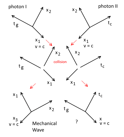
when one of the space dimension has been replaced by a time dimension. The particle exists along the charge time \(t_c\) axis or the gravitational time \(t_g\) axis, from which its velocity is based. And as a wave, travels down the other orthogonal time axis.

\(\cfrac{\partial^2\psi}{\partial\,t^2_c}=\cfrac{\partial\,x}{\partial\,t_c}\cfrac{\partial\,t_g}{\partial\,t_c}\cfrac{\partial^2\psi}{\partial\,t_g\partial\,x}\)

\(\cfrac{\partial^2\psi}{\partial\,t^2_g}=\cfrac{\partial\,x}{\partial\,t_g}\cfrac{\partial\,t_c}{\partial\,t_g}\cfrac{\partial^2\psi}{\partial\,t_c\partial\,x}\)

Since,

\(t_c=\cfrac{1}{\sqrt{2}}t.e^{-i\pi/4}\)  and  \(t_g=\cfrac{1}{\sqrt{2}}t.e^{+i\pi/4}\)

\(t_c=t_ge^{-i\pi/2}\) --- (a)

\(t_c=-it_g\)  and \(\cfrac{\partial\,t_c}{\partial\,t_g}=-i\)

\(t_g=it_c\)  and   \(\cfrac{\partial\,t_g}{\partial\,t_c}=i\)

and,

\(\cfrac{\partial\,x}{\partial\,t_c}=\cfrac{\partial\,x}{\partial\,t_g}=ic\)

this definition of velocity has a explicit direction notation \(i\) to be consistent with the explicit orthogonality between the time axes in (a) above

The equations for 'time' waves are then given by,

\(\cfrac{\partial^2\psi}{\partial\,t^2_c}=ic.i\cfrac{\partial^2\psi}{\partial\,x\partial\,t_g}=ici\cfrac{\partial^2\psi}{\partial\,x\partial\,(it_c)}=ic\cfrac{\partial^2\psi}{\partial\,x\partial\,t_c}\)

\(\cfrac{\partial^2\psi}{\partial\,t^2_g}=ic.(-i)\cfrac{\partial^2\psi}{\partial\,x\partial\,t_c}=ic.(-i)\cfrac{\partial^2\psi}{\partial\,x\partial\,(-it_g)}=ic\cfrac{\partial^2\psi}{\partial\,x\partial\,t_g}\)

from the post "How Time Flies".  \(t_c\) and \(t_g\) are equivalent.  A mass particle is associated with \(t_g\) and an electron is associated with \(t_c\).

Consider the Lagrangian,

\(L=T-V\)

\(\cfrac{d\,}{d\,t}\left(\cfrac{\partial\, L}{\partial\,\dot{x}}\right)=\cfrac{\partial\, L}{\partial\,x}\)

If all dimension are equivalent, then the Lagrangian and Euler-Lagrange Equation is still applicable, when \(t\) is either \(t_c\) or \(t_g\).

\(\psi=T+V=\cfrac{1}{2}m_p\dot{x}^2+V\)

\(L=\cfrac{1}{2}m_p\dot{x}^2-(\psi-\cfrac{1}{2}m_p\dot{x}^2)\)

where \(\psi\) is the total energy between the two space dimensions and \(\dot{x}\) the velocity of the particle.

\(L=m_p\dot{x}^2-\psi\)

We consider existence along \(t_c\),

\(\cfrac{d\,}{d\,t_c}\left(\cfrac{\partial\, L}{\partial\,\dot{x}}\right)=\cfrac{d\,}{d\,t_c}\left(\cfrac{\partial}{\partial\,\dot{x}}\left\{m_p\dot{x}^2-\psi\right\}\right)\)

\(\cfrac { d\,  }{ d\, t_c } \left( \cfrac { \partial \, L }{ \partial \, \dot { x }  }  \right) =\cfrac { d\,  }{ d\, t_c } \left( 2m_{ p }\dot { x } -\cfrac { \partial \psi  }{ \partial \, \dot { x }  }  \right) =2m_{ p }\ddot { x } -\cfrac { \partial  }{ \partial \, \dot { x }  } \left\{ \cfrac { d\, \psi  }{ d\, t_c }  \right\} \)

and,

\(\cfrac{\partial\, L}{\partial\,x}=\cfrac{\partial}{\partial\,x}\left\{m_p\dot{x}^2-\psi\right\}=-\cfrac{\partial\,\psi}{\partial\,x}\)

So,

\(\cfrac { \partial  }{ \partial \, \dot { x }  } \left\{ \cfrac { d\, \psi  }{ d\, t_c }  \right\}=2m_{ p }\ddot { x } +\cfrac{\partial\,\psi}{\partial\,x}\) --- (*)

Differentiate with respect to \(x\),

\(\cfrac { \partial}{ \partial \, x } \left\{ \cfrac { \partial  }{ \partial \, \dot { x }  } \left\{ \cfrac { d\, \psi  }{ d\, t_c }  \right\}  \right\} =\cfrac { \partial ^{ 2 }\psi  }{ \partial \, x\partial \, x } \)

\(\cfrac { \partial  }{ \partial \, \dot { x }  } \left\{ \cfrac { \partial ^{ 2 }\psi  }{ \partial \, t_c\partial \, x }  \right\} =\cfrac { \partial  }{ \partial \, \dot { x }  } \left\{ -\cfrac { i }{c } \cfrac { \partial ^{ 2 }\psi  }{ \partial \, t^{ 2 }_c }  \right\} =\cfrac { \partial ^{ 2 }\psi  }{ \partial \, x^{ 2 } } \)

\(\cfrac { \partial  }{ \partial \, \dot { x }  } \left\{  \cfrac { \partial ^{ 2 }\psi  }{ \partial \, t^{ 2 }_c }  \right\} =ic\cfrac { \partial ^{ 2 }\psi  }{ \partial \, x^{ 2 } } \) --- (b)

but,\(\require{cancel}\)

\(\cfrac { \partial \, \psi  }{ \partial \, x } =\cfrac { \partial \, \psi  }{ \partial \, \dot { x }  }\cancelto{0}{ \cfrac { d\, \dot { x }  }{ d\, x }} +\cfrac { \partial \, \psi  }{ \partial \, t_c } \cfrac { d\, t_c }{ d\, x } \)

So (*) becomes,

\(\cfrac { \partial  }{ \partial \, \dot { x }  } \left\{ \cfrac { d\, \psi  }{ d\, t_c }  \right\} =2m_{ p }\ddot { x } +\cfrac { \partial \, \psi  }{ \partial \, t_c } \cfrac { d\, t _c}{ d\, x } \)

Consider,

\(\cfrac { \partial  }{ \partial \, t_c } \cfrac { \partial  }{ \partial \, \dot { x }  } \left\{ \cfrac { d\, \psi  }{ d\, t_c }  \right\} = \cfrac { \partial  }{ \partial \, \dot { x }  } \left\{\cfrac { \partial ^{ 2 }\psi  }{ \partial \, t^{ 2 } _c}\right\}\)

\(= \cfrac { \partial  }{ \partial \, t_c } \left\{ 2m_{ p }\ddot { x } +\cfrac { \partial \, \psi  }{ \partial \, t _c} \cfrac { d\, t_c }{ d\, x }  \right\} =2m_{ p }\dddot { x } +\cfrac { \partial ^{ 2 }\psi  }{ \partial \, t^{ 2 }_c } \cfrac { d\, t_c }{ d\, x } +\cfrac { \partial \, \psi  }{ \partial \, t_c } \cfrac { \partial  }{ \partial \, t _c} \left\{ \cfrac { 1 }{ \cfrac { d\, x }{ d\, t _c}  }  \right\} \)

\(\cfrac { \partial  }{ \partial \, \dot { x }  } \left\{\cfrac { \partial ^{ 2 }\psi  }{ \partial \, t^{ 2 }_c }\right\}= 2m_{ p }\dddot { x } +\cfrac { \partial ^{ 2 }\psi  }{ \partial \, t^{ 2 }_c } \cfrac { d\, t_c }{ d\, x } -\cfrac { \partial \, \psi  }{ \partial \, t_c } \left\{ \cfrac { 1 }{ \left( \cfrac { d\, x }{ d\, t _c}  \right) ^{ 2 } } \cfrac { d^{ 2 }x }{ d\, t^{ 2 }_c }  \right\} \)

So, since \(ic\) is a constant, substitute in (b)

\(ic\cfrac { \partial ^{ 2 }\psi  }{ \partial \, x^{ 2 } } =2m_{ p }\dddot { x } +\cfrac { \partial ^{ 2 }\psi  }{ \partial \, t^{ 2 }_c } \cfrac { d\, t _c}{ d\, x } -\cfrac { \partial \, \psi  }{ \partial \, t_c } \left\{ \cfrac { 1 }{ \left( \cfrac { d\, x }{ d\, t _c}  \right) ^{ 2 } } \cfrac { d^{ 2 }x }{ d\, t^{ 2 }_c }  \right\}\)

\(ic\cfrac { \partial ^{ 2 }\psi  }{ \partial \, x^{ 2 } } =2m_{ p }\dddot { x } +\cfrac { \partial ^{ 2 }\psi  }{ \partial \, t^{ 2 }_c } \cfrac { 1 }{ \dot { x }  } -\cfrac { \partial \, \psi  }{ \partial \, t _c} \left\{ \cfrac { 1 }{ \dot { x } ^{ 2 } } \ddot { x }  \right\} \)

Rearranging the terms,

\(\ddot { x } \cfrac { \partial \, \psi  }{ \partial \, t_c } =-ic\dot { x } ^{ 2 }\cfrac { \partial ^{ 2 }\psi  }{ \partial \, x^{ 2 } } +\dot { x } \cfrac { \partial ^{ 2 }\psi  }{ \partial \, t^{ 2 }_c } +2m_{ p }\dot { x } ^{ 2 }\dddot { x } \)

If the field forces are constants in time given location \(x\),  \(\dddot { x }=0\)

\(\ddot { x } \cfrac { \partial \, \psi  }{ \partial \, t _c} =-ic\dot { x } ^{ 2 }\cfrac { \partial ^{ 2 }\psi  }{ \partial \, x^{ 2 } } +\dot { x } \cfrac { \partial ^{ 2 }\psi  }{ \partial \, t^{ 2 }_c } \) --- (1)

Consider,

\(\cfrac { \partial ^{ 2 }\psi  }{ \partial \, t^{ 2 } _c} =\cfrac { \partial \,  }{ \partial \, t_c} \left\{ \cfrac { \partial \, \psi  }{ \partial \, t_c }  \right\} =\cfrac { \partial \,  }{ \partial \, x } \left\{ \cfrac { \partial \, \psi  }{ \partial \, t_c }  \right\} \cfrac { d\, x }{ d\, t_c } +\cfrac { \partial \,  }{ \partial \, \dot { x }  } \left\{ \cfrac { \partial \, \psi  }{ \partial \, t_c }  \right\} \cfrac { d\, \dot { x }  }{ d\, t_c } \)

From previously,

\( \cfrac { \partial  }{ \partial \, \dot { x }  } \left\{ \cfrac { d\, \psi  }{ d\, t_c }  \right\} =2m_{ p }\ddot { x } +\cfrac { \partial \, \psi  }{ \partial \, t_c } \cfrac { d\, t_c }{ d\, x } \)

Therefore,

\( \cfrac { \partial ^{ 2 }\psi  }{ \partial \, t^{ 2 }_c } =\cfrac { \partial \,  }{ \partial \, x } \left\{ \cfrac { \partial \, \psi  }{ \partial \, t_c }  \right\} \cfrac { d\, x }{ d\, t_c } +\left\{ 2m_{ p }\ddot { x } +\cfrac { \partial \, \psi  }{ \partial \, t _c} \cfrac { d\, t _c}{ d\, x }  \right\} \cfrac { d\, \dot { x }  }{ d\, t _c} \)

\( \cfrac { \partial ^{ 2 }\psi  }{ \partial \, t^{ 2 }_c } =\cfrac { \partial \,  }{ \partial \, t_c } \left\{ \cfrac { \partial \, \psi  }{ \partial \, x }  \right\} \dot{x} +2m_{ p }\ddot { x } ^{ 2 }+\cfrac { \partial \, \psi  }{ \partial \, t _c} \cfrac { \ddot { x }  }{ \dot { x }  } \)

\(\dot { x } \cfrac { \partial ^{ 2 }\psi  }{ \partial \, t^{ 2 }_c } =\cfrac { \partial \,  }{ \partial \, t_c } \left\{ \cfrac { \partial \, \psi  }{ \partial \, x }  \right\} \dot { x } ^{ 2 }+2m_{ p }\dot { x } \ddot { x } ^{ 2 }+\ddot { x } \cfrac { \partial \, \psi  }{ \partial \, t _c} \)

\( \dot { x } \cfrac { \partial ^{ 2 }\psi  }{ \partial \, t^{ 2 } _c} =\cfrac { \partial \,  }{ \partial \, t _c} \left\{ \cfrac { \partial \, \psi  }{ \partial \, x }  \right\} \dot { x } ^{ 2 }+\ddot { x } \cfrac { \partial \,  }{ \partial \, t _c} \left\{ m_{ p }\dot { x } ^{ 2 } \right\} +\ddot { x } \cfrac { \partial \, \psi  }{ \partial \, t_c } \)

Since,

\( \psi =\cfrac { 1 }{ 2 } m_{ p }\dot { x } ^{ 2 }+V\)

\( m_{ p }\dot { x } ^{ 2 }=2(\psi -V)\)

We have,

\( \dot { x } \cfrac { \partial ^{ 2 }\psi  }{ \partial \, t^{ 2 }_c } =\cfrac { \partial \,  }{ \partial \, t_c } \left\{ \cfrac { \partial \, \psi  }{ \partial \, x }  \right\} \dot { x } ^{ 2 }+2\ddot { x } \cfrac { \partial \,  }{ \partial \, t _c} \left\{ \psi -V \right\} +\ddot { x } \cfrac { \partial \, \psi  }{ \partial \, t_c} \)

\(\dot { x } \cfrac { \partial ^{ 2 }\psi  }{ \partial \, t^{ 2 }_{ c } } =-\cfrac {i }{ c } \cfrac { \partial ^{ 2 }\psi  }{ \partial \, t^{ 2 }_{ c } } \dot { x } ^{ 2 }+2\ddot { x } \cfrac { \partial \,  }{ \partial \, t_{ c } } \left\{ \cfrac { 3 }{ 2 } \psi -V \right\} \)

\(\dot { x } \cfrac { \partial ^{ 2 }\psi  }{ \partial \, t^{ 2 }_{ c } } \left( 1+i\cfrac { \dot { x }  }{ c }  \right) =2\ddot { x } \cfrac { \partial \,  }{ \partial \, t_{ c } } \left\{ \cfrac { 3 }{ 2 } \psi -V \right\} \)

\(\dot { x } \cfrac { \partial ^{ 2 }\psi  }{ \partial \, t^{ 2 }_{ c } } =\cfrac { 2\ddot { x }  }{ \left( 1+i\cfrac { \dot { x }  }{ c }  \right)  } \cfrac { \partial \,  }{ \partial \, t_{ c } } \left\{ \cfrac { 3 }{ 2 } \psi -V \right\} \)

And (1) becomes,

\( \ddot { x } \cfrac { \partial \, \psi  }{ \partial \, t _c} =-ic\dot { x } ^{ 2 }\cfrac { \partial ^{ 2 }\psi  }{ \partial \, x^{ 2 } } +\cfrac { 2\ddot { x }  }{ \left( 1+i\cfrac { \dot { x }  }{ c }  \right)  } \cfrac { \partial \,  }{ \partial \, t _c} \left\{ \cfrac { 3 }{ 2 } \psi -V \right\}\)

\( \ddot { x } \cfrac { \partial \, \psi  }{ \partial \, t_{ c } } \left\{ 1-\cfrac { 3 }{ \left( 1+i\cfrac { \dot { x }  }{ c }  \right)  }  \right\} =-ic\dot { x } ^{ 2 }\cfrac { \partial ^{ 2 }\psi  }{ \partial \, x^{ 2 } } -\cfrac { 2\ddot { x }  }{ \left( 1+i\cfrac { \dot { x }  }{ c }  \right)  } \cfrac { \partial V\,  }{ \partial \, t_{ c } }  \)

\(\ddot { x } \cfrac { \partial \, \psi  }{ \partial \, t_{ c } } \left\{ \cfrac { -2+i\cfrac { \dot { x }  }{ c }  }{ \left( 1+i\cfrac { \dot { x }  }{ c }  \right)  }  \right\} =-ic\dot { x } ^{ 2 }\cfrac { \partial ^{ 2 }\psi  }{ \partial \, x^{ 2 } } -\cfrac { 2\ddot { x }  }{ \left( 1+i\cfrac { \dot { x }  }{ c }  \right)  } \cfrac { \partial V\,  }{ \partial \, t_{ c } }  \)

\(\ddot { x } \left( 2-i\cfrac { \dot { x }  }{ c }  \right) \cfrac { \partial \, \psi  }{ \partial \, t_{ c } } =ic\left( 1+i\cfrac { \dot { x }  }{ c }  \right) \dot { x } ^{ 2 }\cfrac { \partial ^{ 2 }\psi  }{ \partial \, x^{ 2 } } +2\ddot { x } \cfrac { \partial V\,  }{ \partial \, t_{ c } } \) --- (**)

This is not a wave in space and time \(t\).

When \(\ddot{x}=0\),

\(ic\left( 1+i\cfrac { \dot { x }  }{ c }  \right) \dot { x } ^{ 2 }\cfrac { \partial ^{ 2 }\psi  }{ \partial \, x^{ 2 } } =0\)

which implies,

\(\cfrac { \partial ^{ 2 }\psi  }{ \partial \, x^{ 2 } } =0\)

which means,

\(\cfrac { \partial \psi  }{ \partial \, x }=constant=A\) --- (2)

\(\psi(x)=Ax+C\)

\(\psi(x)\) is linear in space!  If at \(x=0\), \(\psi(0)=C=0\)

\(\psi(x)=Ax \)

\(A\) is then a force and we have simply,

\(Energy=\psi(x)=A.x= Force . distance=Work\)

We started with a particle that might be responsible for gravity or electrostatic force and ended with a simple work done equation.  This means the energy of this particle is just work done against a force.
Here the force is given the definition as rate of change of energy, \(\psi\) with distance \(x\), from (2).

When \(\dot{x}=c\),  which is the case for charges, expression (**) becomes,

\(\ddot { x } \left( 2-i \right) \cfrac { \partial \, \psi  }{ \partial \, t_{ c } } =ic^3\left( 1+i \right)\cfrac { \partial ^{ 2 }\psi  }{ \partial \, x^{ 2 } } +2\ddot { x } \cfrac { \partial V\,  }{ \partial \, t_{ c } } \)

\(\ddot { x } \left( 2-i \right) \cfrac { \partial \, \psi  }{ \partial \, t_{ c } } =c^3(-1+i)\cfrac { \partial ^{ 2 }\psi  }{ \partial \, x^{ 2 } } +2\ddot { x } \cfrac { \partial V\,  }{ \partial \, t_{ c } } \)

Comparing real and imaginary parts,

\( 2\ddot { x } \cfrac { \partial \, \psi  }{ \partial \, t_{ c } } =-c^3\cfrac { \partial ^{ 2 }\psi  }{ \partial \, x^{ 2 } } +2\ddot { x } \cfrac { \partial V\,  }{ \partial \, t_{ c } } \) --- (2)

\( -i\ddot { x } \cfrac { \partial \, \psi  }{ \partial \, t_{ c } } =ic^3\cfrac { \partial ^{ 2 }\psi  }{ \partial \, x^{ 2 } } \)

\( \ddot { x } \cfrac { \partial \, \psi  }{ \partial \, t_{ c } } =-c^3\cfrac { \partial ^{ 2 }\psi  }{ \partial \, x^{ 2 } } \)  substitute into (2)

\( \cfrac { \partial \, \psi  }{ \partial \, t_{ c } } =2\cfrac { \partial V\,  }{ \partial \, t_{ c } }  \)  and  \(\cfrac { \partial \, \psi  }{ \partial \, t } =2\cfrac { \partial V\,  }{ \partial \, t }\)

Since, \(\psi=T+V\)

\( \cfrac { \partial \, \psi  }{ \partial \, t_{ c } } =2\cfrac { \partial T\,  }{ \partial \, t_{ c } }  \)  and  \(\cfrac { \partial \, \psi  }{ \partial \, t } =2\cfrac { \partial V\,  }{ \partial \, t }\)

\( \cfrac { \partial \, \psi  }{ \partial \, t_{ c } } \) is divided evenly between \(\cfrac { \partial T\,  }{ \partial \, t_{ c } } \) and \(\cfrac { \partial V\,  }{ \partial \, t_{ c } } \)

From  \(t_c=\cfrac{1}{\sqrt{2}}t.e^{-i\pi/4}\)  and \( \ddot { x } \cfrac { \partial \, \psi  }{ \partial \, t_{ c } }=-c^3\cfrac { \partial ^{ 2 }\psi  }{ \partial \, x^{ 2 } } \)

\( \ddot { x } \cfrac { \partial \, \psi  }{ \partial \, t } =-\cfrac{c^3}{\sqrt{2}}\cfrac { \partial ^{ 2 }\psi  }{ \partial \, x^{ 2 } }e^{-i\pi/4} \)

This expression is unit dimension correct.  However, in space and time \(t\), \(\psi\) is not a wave along \(x\) even when \(\dot{x}=c\).

Hello, Quantum Mechanics!

Continuing from the previous post "Ready Radiator And Flat Heat", we are reminded of the suspicion from the post "Two Faced And Very Flat..." that electrons are flat entities in two dimension.  It is possible that \(\int^{\infty}_{0}{\psi}dx\) being finite, that in space, \(\psi\) manifests as a flat circular disc of finite boundaries.

If a 'time' wave that exist along charge time \(t_c\) manifest in space as a negative charge, the electron, then the same type of wave travelling down the negative charge time axis will be the positive charge.  Both are 2D circular disc particles in space.

In a similar way, the 'time' wave that exist along gravitational time is the gravity particle analogous to an electron, and the same type of wave along the negative gravitational time axis is the anti-mass, anti- gravity particle.  In an analogous way, both particles are flat 2D disc in space.

If at this point, the ideal of heat being a particle that radiates without being at light speed in space is still valid, then heat is the transfer of gravity particles.  Heat is also transferred when there is a movement of charges but we don't confer it as an energy transfer but attribute the resultant heat to ohmic resistance.

This suggestive relationship between heat/energy transfer/energy oscillations and gravity might explain why two hot bodies repel each other, as proposed in the post "\(\tau_o\) The New Guy On The Block";  they are exchanging gravity particles that travel down the negative gravitation time axis, ie anti-gravity particle.

Energy ocillation between two space dimensions of such particles also explains the why a conductor heats up when a current passes through it; electron is in the first place a flow of flat disc particles that have, between two space dimensions in its manifestation, oscillating energy.  So, the space within the conductor heats up and as the electrons pass through.

But such transfer of energy occurs in both ways.  When energy is removed by the electrons as it passes the conducting material will cool.  Thermoelectric cooling employed by a Peltier device is an example of this reversed energy flow.

The 'time' wave it seems is both heat (transfer of energy) and a 2D disc particle.  Hello, Quantum Mechanics!