Equating To A Indefinite Integral

This post is invalid because the post "Into A Pile Of Deep Shit" dated 09 Jun 2016, has been corrected.

\(q=\psi\)

although the discussion of the Lagrangian as Leftover energy is valid.

From the previous post "Into A Pile Of Deep Shit" dated 09 Jun 2016,

\({ q_{a_{\psi}} } =2\dot { x }F_{\rho}|_{a_{\psi}}\)

\(F_{ \rho  }=i\sqrt { 2{ mc^{ 2 } } } \, G.tanh\left( \cfrac { G }{ \sqrt { 2{ mc^{ 2 } } }  } (x-x_{ z }) \right)\) --- (1)

For simplicity, \(x_z=0\) and

\(\cfrac { G }{ \sqrt { 2{ mc^{ 2 } } }  } (a_{\psi})=\pi\)

and

\(tanh\left( \cfrac { G }{ \sqrt { 2{ mc^{ 2 } } }  } (a_{\psi}) \right)=1\) per unit volume

and so,

\({ q_{a_{\psi}} } =i4\pi { \cfrac { \dot { x }  }{ a_{ \psi  } } mc^{ 2 } }\)

where the imaginary sign, \(i\) has been returned and \(i\dot{x}\) is in the direction perpendicular to the radial line along \(a_{\psi}\).  \(i\dot{x}\) is going around a circle with radius along a radial line, in this case the radius is \(x=a_{\psi}\).

\(F_{\rho}\) is force per unit volume, so the term,

\(i\sqrt { 2{ mc^{ 2 } } } \cfrac{\pi}{a_{\psi}} \sqrt { 2{ mc^{ 2 } } }=i2\pi { \cfrac { 1 }{ a_{ \psi  } } mc^{ 2 } }\)

the right hand side of expression (1), is also force per unit volume.  And so,

\({ q_{a_{\psi}} } =2\dot { x }F_{\rho}|_{a_{\psi}}=i4\pi { \cfrac { \dot { x }  }{ a_{ \psi  } } mc^{ 2 } }\)

is power per unit volume.  This is the total power from an conceptual unit sphere centered at the particle.  This power is divided over the surface area of the particle of radius \(a_{\psi}\); this is actually intensity,

\(\cfrac { q_{ a_{ \psi  } } }{ 4\pi \varepsilon _{ o }a^{ 2 }_{ \psi  } } =\cfrac { 1 }{ 4\pi \varepsilon _{ o }a^{ 2 }_{ \psi  } } i4\pi { \cfrac { \dot { x }  }{ a_{ \psi  } } mc^{ 2 } }=i{ \cfrac { \dot { x }  }{ a^{ 3 }_{ \psi  } } \cfrac { mc^{ 2 } }{ \varepsilon _{ o } }  }\)

the power along a radial line when the source is spherical or power per unit area.

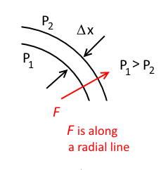
All forces distributed on the uniform sphere except the radial component will cancel; only the radial component of the force associated with this power remains.  Alternatively, given two such power spheres at \(\Delta x\) distance apart at the surface, (ie radii differ by (\(\Delta x\)), a force develops from the higher power sphere to the low power sphere along a radial line.

\(\cfrac{\partial\,F}{\partial\,t}=-\cfrac{\partial\,P}{\partial\,x}\)

This is where we have an extra dimension of "per second", compared to previously when

\(F=\cfrac { q_{a_{\psi}} }{4\pi \varepsilon_o a^2_{\psi} } \)

In the latter, there is no natural resonance frequency and the associated phenomenon of  a body gaining potential energy while in resonance in a field cannot be accounted for.

What happens when we equate,

\(q=4\pi { \cfrac { \dot { x }  }{ a_{ \psi  } } mc^{ 2 } }=4\pi a^2_{\psi}m\) --- (1)

??

When we integrate,

\(F=\int{F_{\rho}}dx\)

where \(F_{\rho}\) is given by (1).

\(F=i2{ mc^{ 2 } }.ln(cosh(\cfrac { G }{ \sqrt { 2{ mc^{ 2 } } }  } (x-x_{ z }))\)

with \(x_z=0\) for simplicity.

\(F\) is the force radiating from a sphere per unit area with radius \(x\), centered at the particle.  This force is along a radial line \(x\).  \(F\) can be interpreted as either force per unit area, or energy (work done) along \(dx\) per unit volume, as \(dx\rightarrow 0\).

When we formulate expression (1),

we are equate the energy change while crossing the spherical boundary of radius \(a_{
\psi}\) with the velocity \(i\dot{x}\), \(\dot{x}\) being along a radius line over an infinitesimal displacement of  \(dx\).  Because, at \(x=a_{\psi}\),

\(\Delta E=\int_{a_{\psi}-\Delta x/2}^{a_{\psi}+\Delta x/2}{F_{\rho}}dx\)

\(\dot{x}=\cfrac{dx}{dt}\)

\(\Delta E=\dot{x}\int_{a_{\psi}-\Delta x/2}^{a_{\psi}+\Delta x/2}{F_{\rho}}\cfrac{dx}{\dot{x}}\)

\(\Delta E=\dot{x}\int_{-\Delta t/2}^{+\Delta t/2}{F_{\rho}}dt\)

\(\Delta E=\dot{x}\left(F_{\rho1}\cfrac{\Delta t}{2}-F_{\rho2}(-\cfrac{\Delta t}{2}) \right)\)

where \(F_{\rho1}\) is \(F_{\rho}\) at \(\cfrac{\Delta t}{2}\) and \(F_{\rho2}\) is \(F_{\rho}\) at \(-\cfrac{\Delta t}{2}\).  As \(\Delta t\rightarrow 0\)

\(F_{\rho1}\rightarrow F_{\rho2}\rightarrow F_{\rho}\)

\(\Delta E=\dot{x}F_{\rho}\Delta t\)

\(\cfrac{\Delta E}{\Delta t}=P=\dot{x}F_{\rho}\)

as \(\Delta t\rightarrow 0\)

Which leads us back to the power, \(P\) per unit volume along \(x\) about \(x=a_{\psi}\).

This invalidates the expression,

\(q=4\pi { \cfrac { \dot { x }  }{ a_{ \psi  } } mc^{ 2 } }=4\pi a^2_{\psi}m\)

because we equated to an indefinite integral that should have been an definite integral along \(x\) between \(x=a_{\psi}-\Delta x/2\) and \(x=a_{\psi}+\Delta t/2\).

\(4\pi { \cfrac { \dot { x }  }{ a_{ \psi  } } mc^{ 2 } }\ne4\pi a^2_{\psi}m\)

but if \(\psi\) of  the system (eg. an uniformly distributed charges over the surface of a conductor) is conserved.

\(i4\pi { \cfrac { \dot { x }  }{ a_{ \psi  } } mc^{ 2 } }=q=constant\)

When we replace \(c\) with \(i\dot{x}\), where we had previously assume light speed,

\(i4\pi { \cfrac { \dot { x } ^3 }{ a_{ \psi  } } m }=-q\)

which suggests a normally negative charge associated with a particle.

\( i\dot { x }^3=-\cfrac{1}{4\pi  }\cfrac{q}{m} a_{ \psi  }\)

\(T=\cfrac{1}{2}m \dot { x }^2\)  Is this true for a wave??

\(\cfrac{\partial\,T}{\partial\,x}=\cfrac{1}{2}m 2.\dot { x }\cfrac{\partial\,\dot{x}}{\partial\,x}\)

\(\cfrac{\partial\,T}{\partial\,x}=m \dot { x }\cfrac{\partial\,\dot{x}}{\partial\,x}\)

\(\cfrac{\partial\,T}{\partial\,x}\) is dependent on \(\dot { x }\).

Normally,

\(\cfrac{\partial\,\dot{x}}{\partial\,x}=0\)

but, \(i\dot{x}\) is perpendicular to \(x\), the change in \(ix\) need not be equal to the change in \(x\) per change in time.  ie,

\(\cfrac{\partial\,i\dot{x}}{\partial\,x}=\dot{\left(\cfrac{\partial\,ix}{\partial\,x}\right)}=\cfrac{\partial}{\partial\,t}\cfrac{\partial\,ix}{\partial\,x}\)

but

\(\cfrac{\partial\,ix}{\partial\,x}\ne 1\)

So,

\(\cfrac{\partial}{\partial\,t}\cfrac{\partial\,ix}{\partial\,x}\ne0\)

this allows the wave \(\psi\) to slow at the boundary,

\(\cfrac { G }{ \sqrt { 2{ mc^{ 2 } } }  } (a_{\psi})=\pi\)

such that,

\({ q_{ a_{ \psi  } } } =3k-2\cfrac { \partial \, T }{ \partial \, x }|_{a_{\psi}}\)

can take on a different sign.  This expression is from the post "Deep Blue Deeper" dated 01 Jun 2016 where,

\(\cfrac{\partial\psi}{\partial x}=\cfrac{\partial V}{\partial x}+\cfrac{\partial T}{\partial x}=k\)

at \(x=a_{\psi}\)

and the post "Why A Positron And Deep Blue..." dated 01 Jun 2016

\(q=\left[3 \cfrac { \partial V\,  }{ \partial \, x } +\cfrac { \partial \, T }{ \partial \, x } \right]_{x=a_{\psi}}\)

Have a nice day.

Note:  The wave \(\psi\) is a also particle, with kinetic and potential energy.  When such a particle enters a field with initial kinetic energy \(T\), all its potential energy is derived from this initial energy \(T\).  What's left of its kinetic energy is,

\(L=T-U\) or \(L=T-V\)

the Lagrangian.

From this \(L\)eftover energy we derive the Lagrange equations of motion from Hamilton’s Principle, which is Newton's law at some level.  \(T\), kinetic energy is the part of the particle's energy in space.   Potential energy is the other part of the particle's total energy in the respective time dimension, \(t_c\), \(t_g\) or \(t_T\).  The particle as a wave has energy oscillating between one space dimension and one of three time dimensions. So,

\(T=\cfrac{1}{2}m \dot { x }^2\)

is true.  What about light speed being constant and light being a wave?

Field Force Per Second...

Flux flow PER SECOND.

which implies everything has three frequencies (one for each field type) and can be set into resonance at each of its three natural resonance frequencies.

And we are closer to answering the question;  Why at resonance of 7.489 Hz gravity particle pushes away from Earth.

Does \(\psi\) accumulates at resonance?

Have a nice day.

Into A Pile Of Deep Shit

From the post "My Own Wave Equation" dated 20 Nov 2014,

\(\left( 1+\cfrac { 1 }{ \gamma ^{ 2 } }  \right) \cfrac { \partial \, \psi  }{ \partial \, t_{ c } } =2\cfrac { \partial V\,  }{ \partial \, t_{ c } } \)

where \(V\) is the potential energy of the particle and \(\cfrac{1}{\gamma^2}=\left( 1-\cfrac { \dot { x } ^{ 2 } }{ c^{ 2 } }  \right)\)

Together with,

\( \psi =T+V\)

we have,

\( \left( 1+\cfrac { 1 }{ \gamma ^{ 2 } }  \right) \cfrac { \partial \, \psi  }{ \partial \, t_{ c } } =2\left( \cfrac { \partial \, \psi  }{ \partial \, t_{ c } } -\cfrac { \partial \, T }{ \partial \, t_{ c } }  \right) \)

\( \left( 1-\cfrac { 1 }{ \gamma ^{ 2 } }  \right) \cfrac { \partial \, \psi  }{ \partial \, t_{ c } } =2\cfrac { \partial \, T }{ \partial \, t_{ c } } \)

\( \left( 1-\cfrac { 1 }{ \gamma ^{ 2 } }  \right) \left(\cfrac { \partial \, \psi  }{ \partial \, t_{ c } } + \cfrac { \partial \, \psi  }{ \partial \, x }\cfrac { \partial \, x }{ \partial \, t_{ c } }\right)=2\left(\cfrac { \partial \, T  }{ \partial \, t_{ c } } + \cfrac { \partial \, T  }{ \partial \, x }\cfrac { \partial \, x }{ \partial \, t_{ c } }\right) \)

For \( \cfrac { \partial \, x }{ \partial \, t_{ c } } \ne 0\),  and \(\cfrac { \partial \, \psi  }{ \partial \, t_{ c } }=0\) as \(\psi\) is stationary, \(\left.\psi\right|_{x}=k\) given \(x\),

\( \left( 1-\cfrac { 1 }{ \gamma ^{ 2 } }  \right) \cfrac { \partial \, \psi  }{ \partial \, x }=2\left(\cfrac { \partial \, T  }{ \partial \, t_{ c } } + \cfrac { \partial \, T  }{ \partial \, x }\cfrac { \partial \, x }{ \partial \, t_{ c } }\right) \cfrac { \partial \, t_{ c } }{ \partial \, x } \)

Here, given a position \(x\), both \(\psi\) do not change through time \(t_c\) but changes along \(x\) as we pass by with \(\dot{x}=\cfrac { \partial \, x }{ \partial \, t_{ c } }\) through fields of stationary values of \(\psi\).

\( \left( 1-\cfrac { 1 }{ \gamma ^{ 2 } }  \right) \cfrac { \partial \, \psi  }{ \partial \, x } =4\cfrac { \partial \, T }{ \partial \, x } \)

Similarly,

\( \left( 1+\cfrac { 1 }{ \gamma ^{ 2 } }  \right) \cfrac { \partial \, \psi  }{ \partial \, x } =4\cfrac { \partial V\,  }{ \partial \, x } \)

With these we take a good hard look at,

\(\cfrac { dq }{ dx } =\left( \cfrac { 3\gamma ^{ 2 }+1 }{ \gamma ^{ 2 }+1 }  \right) \cfrac { \partial V\,  }{ \partial \, x } +\cfrac { \partial \, T }{ \partial \, x }\)

where \(2\left( 1+\cfrac { 1 }{ \gamma ^{ 2 } }  \right) ^{ -1 }+1=\left( \cfrac { 3\gamma ^{ 2 }+1 }{ \gamma ^{ 2 }+1 }  \right)\)

\(\cfrac { dq }{ dx } =\left( \cfrac { 3\gamma ^{ 2 }+1 }{ \gamma ^{ 2 }+1 }  \right) .\cfrac { 1  }{ 4 } \left( 1+\cfrac { 1 }{ \gamma ^{ 2 } }  \right) \cfrac { \partial \, \psi  }{ \partial \, x } +\cfrac { 1  }{ 4 } \left( 1-\cfrac { 1 }{ \gamma ^{ 2 } }  \right) \cfrac { \partial \, \psi  }{ \partial \, x } \)

\( \cfrac { dq }{ dx } =\left( 2\left( 1+\cfrac { 1 }{ \gamma ^{ 2 } }  \right) ^{ -1 }+1 \right) .\cfrac { 1  }{ 4 } \left( 1+\cfrac { 1 }{ \gamma ^{ 2 } }  \right) \cfrac { \partial \, \psi  }{ \partial \, x } +\cfrac { 1 }{ 4 } \left( 1-\cfrac { 1 }{ \gamma ^{ 2 } }  \right) \cfrac { \partial \, \psi  }{ \partial \, x } \)

\( \cfrac { dq }{ dx } = \left( \cfrac{1}{2}+\cfrac { 1 }{ 4} \left( 1+\cfrac { 1 }{ \gamma ^{ 2 } }  \right) +\cfrac { 1 }{ 4 } \left( 1-\cfrac { 1 }{ \gamma ^{ 2 } }  \right)  \right) .\cfrac { \partial \, \psi  }{ \partial \, x } \)

\( \cfrac { dq }{ dx } =\cfrac { \partial \, \psi  }{ \partial \, x } = \cfrac { d\psi }{ dx }\)

as \(\psi\) is independent of \(t_c\) given \(x\),

\(q=\psi\)

which is the reason we needed in the post "Why A Positron And Deep Blue..." dated 01 Jun 2016, for the expression,

\(\cfrac{dq}{dx}=\cfrac{\partial\,\psi}{\partial\,t}\cfrac{\partial\,t}{\partial\,x}+\cfrac{\partial\,\psi}{\partial\,x}\)

and we don't have problem with this.

Field Equation Exponential Form

From the post "May The Hunt Begin" dated 01 Jun 2016,

We know that \(\Delta q\) decreases to zero at \(r=a_{\psi}\), as such,

\(-\Delta q=m.4\pi r^{ 2 }.\Delta r\)

\({q}=m.4\pi a^2_{\psi}=- \cfrac { dq }{ d\,r}|_{r=a_{\psi} }\)

previously \(q\) has retained the minus sign.  If we solve for

\( \cfrac { dq }{ d\,r }=-q\)

we have,

\(\int { \cfrac { 1 }{ q }  } dq=\int { -1} dr\)

\(ln(q)+C= -r+B\)

\(ln(Aq)= -( r-D) \)

\(Aq=e^{- (r-D ) }\)

\(q=E.e^{-(r-D )}\)

where at \(r=a_{\psi}\),  \(\cfrac { dq }{ d\,r}|_{r=a_{\psi} }=-q_{a_{\psi}}\)

we let \(D=a_{\psi}\),  \(E={q_{a_{\psi}}}\)

\(q=q_{a_{\psi}}.e^{-(r-a_{\psi}) }\)

\(\because\)

\(\cfrac { dq }{ d\, r } =q_{ a_{ \psi  } }.e^{ -(r-a_{ \psi  }) }=-q\)

And,

\(\cfrac { q }{ \varepsilon _{ o } } =\cfrac { q_{ a_{ \psi  } } }{ \varepsilon _{ o } } e^{(r-a_{ \psi  }) }\)

This is the change in flux \(\cfrac { q }{ \varepsilon _{ o } }\) along a radial line \(r\), which is also the Newtonian force along the line joining two particles center to center.

It is the change in \(q\), not \(q\) itself but \(\Delta q\) decreasing at \(r=a_{\psi}\) that invites a minus sign in the exponent of the expression for force in exponential form.

The direction of the force in expression (*) depends on the sign of \(q_{a_{\psi}}\) or \(q\).

This expression will satisfy the wave equation, whereas the expression,

\(F_{\small{G}}\cfrac{1}{4\pi a^2_{\psi}}=\cfrac{q}{4\pi\varepsilon_o a^2_{\psi}}=2{ mc^{ 2 } }.ln(cosh(\pi))\)

does not; as shown previously.

Expression (*) should be interpreted as the decreasing effects of \(q\) over \(r\) beyond \(r=a_{\psi}\) and not the spread of \(q\) beyond \(a_{\psi}\).  The particle extends up to \(r=a_{\psi}\) and ends abruptly, the gradient of which is given by,

\( \cfrac { dq }{ d\,r }=-q\)

And the force is exponential.  May the force extends beyond you exponentially.

The Iris

This might speed up the dialing process,

where three circular portals rotated to cover a sphere, operate together with an iris opening for access.

Have a nice day.

Found It! Treasures In A Dumpster

A small portal to dump electrons,

is an infinite source of energy.

For infinite gain, all that matters is what and where to throw away.  Throwing electrons into a small portal.

Have a nice day.

Deep Blue Deeper

From the previous post "Why A Positron And Deep Blue..." dated 1 Jun 2016,

\({q}=\left[3 \cfrac { \partial V\,  }{ \partial \, x } +\cfrac { \partial \, T }{ \partial \, x } \right]_{x=a_{\psi}}.a_{\psi}\)

For a spread of \(\psi\) around a center,

\(\cfrac{\partial\psi}{\partial x}=\cfrac{\partial V}{\partial x}+\cfrac{\partial T}{\partial x}=k\)  at a particular value of \(x=a_{\psi}\) ie.

\(\cfrac{\partial\psi}{\partial t}|_{x=a_{\psi}}=0\)

\(k\) is a constant for stationary (in time) fields, where a particle passing through a particular point \(x\), will always have the same \(V\) and \(T\) values.  We have

\(\cfrac{q}{a_{\psi}}=2\cfrac { \partial \, V }{ \partial \, x }|_{a_{\psi}}+k\)

We have maximum when \(\cfrac { \partial \, V }{ \partial \, x }|_{a_{\psi}}\) is maximum.

If \(\dot{x}=c\) is a constant at light speed, then \(\cfrac { \partial \, T }{ \partial \, x }\) is also a constant, zero, so,

\(\cfrac{\partial\psi}{\partial x}=\cfrac{\partial V}{\partial x}\)

which means,

\(\cfrac{q}{a_{\psi}}=3\cfrac { \partial \, \psi }{ \partial \, x }|_{a_{\psi}}\)

and \(q\) is still quantized.  What is interesting is,

\(\cfrac{q}{a_{\psi}}=3k-2\cfrac { \partial \, T }{ \partial \, x }|_{a_{\psi}}\)

If \(T\) is lowered very quickly,

\(\cfrac { \partial \, T }{ \partial \, x }|_{a_{\psi}}\rightarrow -\infty\)

then

\(\cfrac{q}{a_{\psi}}\rightarrow \infty\)

If we still insist on,

\(\cfrac{\partial\psi}{\partial x}=\cfrac{\partial V}{\partial x}+\cfrac{\partial T}{\partial x}=k\)

(ie. the particle not breaking up) then,

\(\cfrac{\partial V}{\partial x}|_{a_{\psi}}\rightarrow \infty\)

\(F_{n}=\cfrac{\partial V}{\partial x}|_{a_{\psi}}\) is a force orthogonal to \(\cfrac { \partial \, T }{ \partial \, x }|_{a_{\psi}}\).  If the latter is around a circle, then \(F_{n}\) is perpendicular to the circle through its center.

But where is this force driving us?  Through time.

How to slow down \(\psi\)?  \(f_{res}=2.870\,\,Hz\)! From the post "A Shield" dated 27 may 2016. On Earth, because Earth is also one big charge particle.

It is still dream land, only deeper...sleep on this,

Good night.

Why A Positron And Deep Blue...

From the post "May the Hunt Begin" dated 1 Jun 2016,

\(q=m.4\pi a^2_{\psi}= \cfrac { dq }{ dx }|_{x=a_{\psi}}\)

Given an example of a particle with a surrounding field,

\(a_{\psi}\) is along \(x\) in the diagram.  So,

\(\cfrac{dq}{dx}=\cfrac{\partial\,\psi}{\partial\,t}\cfrac{dt}{dx}+\cfrac{\partial\,\psi}{\partial\,x}\)

since there is no other entity in this model other than \(\psi\), which is a big assumption here.

\(\cfrac{dq}{dx}=\cfrac{1}{c}\cfrac{\partial\,\psi}{\partial\,t}+\cfrac{\partial\,\psi}{\partial\,x}\)

when the particle exist along \(t_c\),

\(\cfrac{dq}{dx}=\cfrac{1}{c}\cfrac{\partial\,\psi}{\partial\,t_c}+\cfrac{\partial\,\psi}{\partial\,x}\)

From the post "My Own Wave Equation" dated 20 Nov 2014,

\(\left(1+\cfrac{1}{\gamma^2} \right)\cfrac { \partial \, \psi  }{ \partial \, t_{ c } }=2\cfrac { \partial V\,  }{ \partial \, t_{ c } }\)

where \(V\) is the potential energy of the particle and \(\cfrac{1}{\gamma^2}=\left( 1-\cfrac { \dot { x } ^{ 2 } }{ c^{ 2 } }  \right)\)

We have,

\(\cfrac{dq}{dx}=\cfrac{2}{c}\left(1+\cfrac{1}{\gamma^2} \right)^{-1}.\cfrac { \partial V\,  }{ \partial \, t_{ c } }+\cfrac{\partial\,\psi}{\partial\,x}\)

Assuming that \(V\) is stationary in space and changes only because of the particle is at velocity \(c\),

\(\cfrac { dq }{ dx } =\cfrac { 2 }{ c } \left( 1+\cfrac { 1 }{ \gamma ^{ 2 } }  \right) ^{ -1 }.\cfrac { \partial V\,  }{ \partial \, x } \cfrac { \partial x }{ \partial \, t_{ c } } +\cfrac { \partial \, \psi  }{ \partial \, x } \)

\( \cfrac { dq }{ dx } =2\left( 1+\cfrac { 1 }{ \gamma ^{ 2 } }  \right) ^{ -1 }.\cfrac { \partial V\,  }{ \partial \, x } +\cfrac { \partial \, \psi  }{ \partial \, x } \)

Since,  \(\psi =T+V\) is the total energy,  \(T\) is the kinetic energy,

\( \cfrac { dq }{ dx } =\left( \cfrac { 3\gamma ^{ 2 }+1 }{ \gamma ^{ 2 }+1 }  \right) \cfrac { \partial V\,  }{ \partial \, x } +\cfrac { \partial \, T }{ \partial \, x } \)

\(\cfrac{1}{\gamma^2}\rightarrow 0\),  \(\dot{x}=c\)

\( \cfrac { dq }{ dx } =3 \cfrac { \partial V\,  }{ \partial \, x } +\cfrac { \partial \, T }{ \partial \, x } \)

\({q}=\left[3 \cfrac { \partial V\,  }{ \partial \, x } +\cfrac { \partial \, T }{ \partial \, x } \right]_{x=a_{\psi}}.a_{\psi}\)

\(\psi\) is a wave in the \(ix\) direction, both \(\cfrac { \partial\,V  }{ \partial \, x }\) and \(\cfrac { \partial\, T  }{ \partial \, x }\) are along the radial line, in the \(x\) direction.

\(\cfrac { \partial\,V  }{ \partial \, x }\) represents a force inside the particle,

\(F_{n}=\cfrac { \partial\,V  }{ \partial \, x }\)

that pulls \(\psi\) to the particle center \(x=0\), when \(V\) decreases with \(x\).  When the total \(\psi\) along \(x\) is conserved then, at \(x=a_{\psi}\),

\({q}\gt0\)

when 

 \(3\cfrac { \partial\,V  }{ \partial \, x }|_{a_{\psi}}\gt-\cfrac { \partial\,T  }{ \partial \, x }|_{a_{\psi}}\) 

and,

\({q}\lt0\)

when 

 \(3\cfrac { \partial\,V  }{ \partial \, x }|_{a_{\psi}}\lt-\cfrac { \partial\,T  }{ \partial \, x }|_{a_{\psi}}\)

Without an external force, \(\cfrac { \partial\,V  }{ \partial \, x }|_{a_{\psi}} \) and \(\cfrac { \partial\,T  }{ \partial \, x }|_{a_{\psi}}\) are expected to change in opposite direction, but,

 \(\cfrac { \partial\,\psi  }{ \partial \, x }|_{a_{\psi}}\ne0\)

so,

 \(\cfrac { \partial\,V  }{ \partial \, x }|_{a_{\psi}}\ne-\cfrac { \partial\,T  }{ \partial \, x }|_{a_{\psi}}\)

as \(\psi=V+T\).

The sign of the particle can change!  Either there is a positive electron charge that in spin produces a \(B\) or \(T\) field or positive and negative particles are not differentiated by their oscillating energies.

The former is likely because a positron is known to exist, but borne here, it is not an antimatter.

And of the six particles in total, now we have eighteen, because

\(3\cfrac { \partial\,V  }{ \partial \, x }|_{a_{\psi}}=-\cfrac { \partial\,T  }{ \partial \, x }|_{a_{\psi}}\)

\({q}=0\)

creates a charge neutral particle and makes three possibilities in total for each particle.

This requires a rethink...in deep blue.

May The Hunt Begin

If,

\(q=m.4\pi a_{\psi}^{ 2 }\)

from the post "Pound To Rescue Permittivity" dated 30 May 2016, also,

\(\cfrac{q}{\varepsilon_o}=4\pi a^2_{\psi}m.2c^2ln(cosh(\pi))\)

\(\varepsilon_o\) resists the spread of \(q\) into the region with permittivity, \(\varepsilon_o\).

If each charge is a portal to a storage of flux, \(\varepsilon_o\) resist or aid (\(\varepsilon_o\lt 1\)) the flow of flux from the storage.

\(\cfrac{q}{\varepsilon_o}=q.2c^2ln(cosh(\pi))\)

\(\cfrac{1}{\varepsilon_o.2ln(cosh(\pi))}=c^2\)

And we start a treasure hunt!

Note:  This posts has lost its original meaning.  What was it about?  \(ln(cosh(\pi))\) is arbitrary.  For a basic particle this could be,

\(ln(cosh(\cfrac { G }{ \sqrt { 2{ mc^{ 2 } } }  }a_{\psi\,c}))=\cfrac{1}{4}\)

\(ln(cosh(0.7369))=\cfrac{1}{4}\)

Pound To Rescue Permittivity

From the post "Wrong, Wrong, Wrong" dated 25 May 2015,

\(F=\int{F_{\rho}}dx\)

where  \(F_{ \rho  }=i\sqrt { 2{ mc^{ 2 } } } \, G.tanh\left( \cfrac { G }{ \sqrt { 2{ mc^{ 2 } } }  } (x-x_{ z }) \right)\)

\(F=2{ mc^{ 2 } }.ln(cosh(\cfrac { G }{ \sqrt { 2{ mc^{ 2 } } }  } (x-x_{ z }))\)

within the boundary of \(\psi\) where \(0\le x \le a_{\psi}\).  For, \(x\ge a_{\psi}\), we use Gaussian flux,

\(F=F_{\small{G}}\cfrac{1}{4\pi r^2}\)

at \(r=a_{\psi}\)

\(F_{\small{G}}\cfrac{1}{4\pi a^2_{\psi}}=\cfrac{q}{4\pi\varepsilon_o a^2_{\psi}}=2{ mc^{ 2 } }.ln(cosh(\pi))\)

for a point mass \(x_z=0\) (in retrospect \(x_z\) was not necessary, \(x_z\) was to prevent the function \(F_{\rho}\) from blowing up at \(x=0\)).

\(F_{ { G } }=8mc^{ 2 }\pi a^{ 2 }_{ \psi  }.ln(cosh(\pi ))\)

where \(ln(cosh(\pi))=2.4503\).

Also,

\(\cfrac{q}{\varepsilon_o}=4\pi a^2_{\psi}m.2c^2ln(cosh(\pi))\)

where \(m\) is a point mass/inertia in the respective field.  Which suggests,

\(\varepsilon_o=\cfrac{1}{2c^2ln(cosh(\pi))}=\cfrac{1}{2*299792458^2*ln(cosh(\pi))}\)

\(\varepsilon_o=2.2704e-18\)

when

\(q=4\pi a^2_{\psi}m\)

That \(q\) is the distribution of \(m\) on the surface of a sphere of radius \(a_{\psi}\).  Which seems to solve the problem of extending a point mass of mass density \(m\) to a mass of finite extent \(a_{\psi}\).

But, the quoted value of \(\varepsilon_o\) is \(8.8542e-12\) from the definition,

\(\varepsilon_o=\cfrac{1}{\mu_oc^2}\)

where \(\mu_o=4\pi \times 10^{-7}\)

we have \(4\pi\approx12.5664\) vs \(2ln(cosh(\pi))\approx4.9006\) and a scaling factor of \(10^{-7}\).

The derived \(\varepsilon_o\) and defined value do not match.

A Big Temperature Particle

From the post "A \(\Psi\) Gun" dated 31 May 2016,

\(f_{res}=0.061\cfrac { c }{ a_{\psi} }\)

If the Sun is one big temperature particle,

\(a_{\psi}=695700000\)

\(f_{res}=0.061*299792458/695700000=0.026286\)

which is a period of \(1/0.026286=38.043s\)

What happen to the Sun every 38.0 seconds?

Given,

\(G=\cfrac{\pi \sqrt { 2{ mc^{ 2 } } }  }{a_{\psi}}\)

\(m_{sun}=1.989e30\)

\(G=\cfrac{\pi \sqrt { 2* 1.989e30*299792458^{ 2 }  }  }{695700000}\)

\(G=2.7001e15\)

None of the \(G\) values matches up.  If \(m\) is to be mass density,

\(G_v=\cfrac{\sqrt{3}G}{\sqrt{4\pi a^3_{\psi}}}\)

\(G_v=7.1895e1\)

and we apply a similar CORRECTION to the previous values;

for the case of an electron,

\(G_v=4.511e8*\cfrac{\sqrt{3}}{\sqrt{4\pi* (2.8179403267e−15)^3}}\)

\(G_v=1.474e30\)

and Earth,

\(G_v=5.109e14*\cfrac{\sqrt{3}}{\sqrt{4\pi*(6371e3)^3}}\)

\(G_v=1.552e4\)

The values still do not match up.  \(m\) is the mass of a point particle.

\(m=\cfrac{\Delta M}{\Delta V}=\cfrac{dM}{dV}\)  as \(\Delta V\rightarrow 0\)

the condition \(\Delta V\rightarrow 0\) applies for the fact that \(m\) is a point.

When the mass is not a point mass, \(m\) is the total mass of the particle because the force involved acts on the total mass of the particle.

X Ray, Inner Electron Cloud And Just As Shocking

From the post "A Shield" and "A \(\Psi\) Gun" both dated 27 May 2016,

\(f_{res}=0.061\cfrac { c }{ a_{\psi} }\)

\(a_{\psi}\) is driven to oscillate about \(x=\cfrac{\pi \sqrt { 2{ mc^{ 2 } } }  }{G}\).  The work done in moving \(\psi\) forward is given by,

\(\int_{\pi-A_w}^{\pi+A_p}{tanh(x)}dx\)

On the return, at position \(x\), \(\psi\) radiates this energy gained.  The energy radiated is,

\(X=\int_{\pi-A_w}^{\pi+A_p}{tanh(x)}dx-\int_{\pi-A_w}^{x}{tanh(x)}dx\)

\(X=\left[ ln(cosh(x)) \right] _{ \pi -A_{ w } }^{ \pi +A_{ p } }-\left[ ln(cosh(x)) \right] _{ \pi -A_{ w } }^{ x }\)

\( X=X_{ o }-ln(cosh(x))\)

with,   \( X_{ o }=ln(cosh(\pi +A_{ p }))\)

A plot of log(cosh(pi+2))-log(cosh(x)) shows an almost linear decrease in energy radiated given the position \(x=a_{\psi}\),

\(U_{1/2}\) marks the value of \(a_{\psi}\) where work done travelling on the left and right side are equal.

We would also expect an almost linear increase in \(X\) as the amplitude \(A_p\) is increased at any given position, for example \(x=\pi\). ie

\( X_{\pi}=ln(cosh(x_{1/2} +x))-ln(cosh(x_{1/2}))\)

is almost increasing linearly.  In addition, when \(a_{\psi}\) drops below

\(n.2\pi f_n a_{\psi}=c\) --- (*)

where the particle(s) is in resonance along \(2\pi a_{\psi}\) with \(n\) wavelengths along the perimeter of a circle of radius \(a_{\psi}\), a radiation peak occurs as \(a_{\psi}\) move to a lower energy state \(n-1\).

\(a_{\psi}\) is driven to a higher value above \(x=\cfrac{\pi \sqrt { 2{ mc^{ 2 } } }  }{G}\) by an external field, on its return, it travels below it normal energy state.  It loses energy continuously, when it passes a resonance point given by (*), it emits an resonance peak.  This is not the energy states given by the Schrodinger wave equation of orbiting electrons, they are energy states when two or more particles interacting as waves exist in a cloud of energy density, \(\psi\), from the post "Two Quantum Wells, Quantum Tunneling, \(v_{min}\)" dated 19 Jul 2015.  In particular, the driving field is affecting the inner electron clouds that surrounds the nucleus below the orbiting \(T^{+}\) particles as described in the post "The Rest Are In The Clouds" dated 16 Apr 2016.

The following table is the X ray emission data using high energy electron bombardment,

Element	ave \(E\,\alpha\)	\(E\,\alpha1\)	\(E\,\alpha2\)	\(E\,\beta\)	n	\(a_{\psi}1\)	\(a_{\psi}2\)
Cr2,8,13,1	2.29100	2.28970	2.29361	2.08487	11	0.0331517775	0.0331858844
Fe2,8,14,2	1.93736	1.93604	1.93998	1.75661	10	0.0308378963	0.0310675679
Co2,8,15,2	1.79026	1.78897	1.79285	1.62079	10	0.0284964345	0.0286654428
Cu2.8.18.1	1.54184	1.54056	1.54439	1.39222	9	0.0272691257	0.0277007991
Mo2,8,18,13,1	0.71073	0.70930	0.71359	0.63229	8	0.0141412915	0.0143778083

\(a_{\psi}1\) and \(a_{\psi}2\) are calculated data.

The split into \(E\,\alpha1\) and \(E\alpha2\) is consistent with the split in the solution for \(a_{\psi}\) in the post "Two Quantum Wells, Quantum Tunneling, \(v_{min}\)" dated 19 Jul 2015.  \(E \beta\) is due to the energy state available at the next lower level, \(n-1\).

We estimate the value of \(n\) and the next lower energy state \(n-1\) by taking the ratio of,

\(\cfrac{ave.\,E\alpha}{E\beta}=\cfrac{n}{n-1}\)

since,

\(n.2\pi a_{\psi}=\cfrac{c}{f_n}=\lambda_n\)

\(\cfrac{\lambda_n}{\lambda_{n-1}}=\cfrac{n}{n-1}\)

Using the average value of \(E\alpha1\) and \(E\alpha2\) and \(E\beta\) to find \(a_{\psi1}\) and \(a_{\psi2}\) respectively.

\(a_{\psi}=\cfrac{\lambda_n}{n.2\pi }\)

For \(Cu\), the inner electron cloud has a radius of \(a_{\psi}=0.02447*10^{-10}\)

which is one fifth the size of the atomic radius at 1.45 A.  This lead us to the resonance frequency,

\(f_{res}=0.061\cfrac { 299792458 }{ 0.02447*10^{-10}}=7.473*10^{18} Hz=7.473 EHz\)

needed to drive \(a_{\psi}\) to resonance.  Given an elementary electron charge of 1.602176565*10^{-19} C, a bombardment at \(f_{res}\) is

\(I_{res}=q_e.f_{res}=1.602176565*10^{-19}*7.473*10^{18}=1.1974 A\)

This radiation due to the excitation of the inner electron clouds is in the \(X\) ray region.  If this is true, with \(f_{res}\), \(X\) ray production is safer and cheaper... Hurrah!  Just before you electrocute yourself, that's 1.1974 A per electron cloud.  Hurrah!

The good news is any integer division of \(f_{res}\) will still set the system into resonance but slowly. For example,

\(f=\cfrac{f_{res}}{1000}\)

will still resonate but has a slow buildup.

Note:  As the atomic size increases the inner electron cloud is compressed to a smaller radius.

A \(\Psi\) Gun

If we express \(f_{res}\) in terms of \(a_{\psi}\), the extend of \(\psi\),

\(a_{\psi}=\cfrac{\pi \sqrt { 2{ mc^{ 2 } } }  }{G}\)

\(f_{res}=\cfrac{sech(\pi)}{2\pi}\cfrac{G}{\sqrt{m}}=\cfrac { sech(\pi ) }{ 2 } \cfrac { \sqrt { 2{ c^{ 2 } } }  }{ a_{\psi} }  \)

\(f_{res}=\cfrac { \sqrt { 2 }  }{ 2 } sech(\pi )\cfrac { c }{ a_{\psi} }\)

\(f_{res}=0.061\cfrac { c }{ a_{\psi} }\)

Does the system work in reverse?  Once \(\psi\) is set into resonance, and \(f_{res}\) is reduced does \(a_{\psi}\) increases.

Can a shield be projected forward by suddenly decreasing \(f_{res}\) and turning off.  In effect, an energy density \(\psi\) projectile.

And I continue to dream anime...   看\(\psi\)！

A Shield

The three plots of \(F_{\rho}\), \(F^{'}_{\rho}\) and \(F^{''}_{\rho}\) are provided below,

in the case of a simple spring-particle system, the force from the retaining spring changes direction and reverses the travel direction of the attached particle.  The particle's motion is periodic and oscillatory.  In the case of a particle held by a field, the nature of the particle's interaction with the field as a particle or as a wave changes the direction of the force.  The field is negative and attracts the particle beyond \(\pi\), as the particle returns below \(\pi\) it is repelled by the field as a wave and is eventually pushed out towards \(\pi\) again.

When the particle is oscillating, energy is conserved,

\(\int_{\pi-A_w}^{\pi}{tanh(x)}dx=\int_{\pi}^{\pi+A_p}{tanh(x)}dx\)

Solving,

\(\int _{ \pi -A_{ w } }^{ \pi  }{ tanh(x) } dx=\int _{ \pi  }^{ \pi +A_{ p } }{ tanh(x) } dx\)

\( \left[ ln(cosh(x)) \right] _{ \pi -A_{ w } }^{ \pi  }=\left[ ln(cosh(x)) \right] _{ \pi  }^{ \pi +A_{ p } }\)

\( ln(cosh(\pi ))-ln(cosh(\pi -A))=ln(cosh(\pi +A))-ln(cosh(\pi ))\)

\( 2ln(cosh(\pi ))-ln(cosh(\pi -A_{ w }))=ln(cosh(\pi +A_{ p }))\)

\( 2ln(cosh(\pi ))=ln(cosh(\pi +A_{ p })cosh(\pi -A_{ w }))\)

\( cosh^{ 2 }(\pi )=cosh(\pi +A_{ p })cosh(\pi -A_{ w })\)

\(cosh(\pi -A_{ w })=\cfrac { cosh^{ 2 }(\pi ) }{ cosh(\pi +A_{ p }) } \)

A plot of cosh(pi)*cosh(pi)/cosh(pi+x) and cosh(pi-x) gives,

where valid solutions to \(A_w\) and \(A_p\) share a common value on the y-axis.

It is interesting that a valid solution swings the particle within the boundary of \(-\pi\) and \(\pi\) across the center of \(\psi\).

And the thickness of this shield is \(A_w+A_p\).

The actual expression for \(F_{\rho}\) the post "Not Exponential, But Hyperbolic And Positive Gravity!" dated 22 Nov 2014 is,

\(F_{ \rho  }=i\sqrt { 2{ mc^{ 2 } } } \, G.tanh\left( \cfrac { G }{ \sqrt { 2{ mc^{ 2 } } }  } (x-x_{ z }) \right)\)

\(\cfrac{\partial\,F_{\rho}}{\partial\,x}=G^2sech^2(\cfrac { G }{ \sqrt { 2{ mc^{ 2 } } }  }x)\)

where we let \(x_z=0\), ie a point particle, and ignore \(i\),

at \(\cfrac { G }{ \sqrt { 2{ mc^{ 2 } } }  }x=\pi\)    or,

\(x=\cfrac{\pi \sqrt { 2{ mc^{ 2 } } }  }{G}\)

we approximate \(f_{res}=\cfrac{1}{2\pi}\sqrt{\cfrac{gradient|_{\pi}}{m}}=\cfrac{1}{2\pi}\sqrt{\cfrac{G^2sech^2(\pi)}{m}}\)

 \(f_{res}=\cfrac{sech(\pi)}{2\pi}\cfrac{G}{\sqrt{m}}=0.01373\cfrac{G}{\sqrt{m}}\)

where \(m\) is the mass of the particle.

From the same post "Not Exponential, But Hyperbolic And Positive Gravity!" dated 22 Nov 2014,  \(G\) has the same dimension (units) as \(\sqrt{2mc^2}\) per meter, the expression for \(f_{res}\) has a consistent unit of per second.  But without an estimate for \(G\) it is useless.

If the radius of an electron is

\(a_e=2.8179403267e-15 m\)

and its mass

\(m=9.10938291e-31 kg\)

and that the \(\psi\)  of an electron extend up to \(a_e\) then,

\(a_e=\cfrac{\pi \sqrt { 2{ mc^{ 2 } } }  }{G}\)

\(G=\cfrac{\pi \sqrt { 2{ mc^{ 2 } } }  }{a_e}\)

\(G=4.511e8\)

So, in the case of an electron,

 \(f_{res}=0.01373\cfrac{G}{\sqrt{m}}=0.01373\cfrac{4.511e8}{\sqrt{9.10938291e-31}}\)

 \(f_{res}=6.489e21 Hz\)

We can still achieve resonance at integer division of this number although slow, but this shield is just the size of an electron.

In the case of Earth as one big gravity particle,

\(a_E=6371e3m\)

and mass

\(m_E=5.972e24 kg\)

\(G\)=pi*sqrt(2*5.972*(299792458)^2*10^(24))/(6371e3)

\(G=5.109e14\)  and

\(f_{res}\)=0.01373*5.109e14/sqrt(5.972e24)

\(f_{res}=2.870\,\,Hz\)

on the surface of earth.

This frequency can be reproduced.

Good luck!  And I dream of anime...ZZZ...

Note: Newton Gravitational Constant \(G=6.67408*10^{-11}\),

\(GM_E=6.67408*10^{-11}*5.972*10^{24}\)

\(GM_E=3.9858*10^{14}\)

A Shield Forming...Heat Dispersion

If the temperature particles are interacting as waves, what is the difference between a \(B\) field and a \(T\) field?  Moving electron generates a \(B\) field.  The field around a temperature particle is a \(T\) field.  Which points us the the magic value \(\pi\).

Temperature particles interact within \(2\pi\) range of the force density, \(F_{\rho}\).  This is the \(T\) field.  \(B\) field is interaction beyond the \(2\pi\) range centered about zero.  \(B\) and \(T\) fields are the same \(F_{\rho}\) but are at different ranges.

Within  the respective ranges,  force density \(F_{\rho}\) is such that,

\(F_{\rho}\ge0\),   \(\cfrac{\partial F_{\rho}}{\partial\,x}=+ve\) and \(\cfrac{\partial^2F_{\rho}}{\partial\,x^2}=-ve\)

make like particle attract each other.  And

\(F_{\rho}\gt0\),   \(\cfrac{\partial F_{\rho}}{\partial\,x}=0\) and \(\cfrac{\partial^2F_{\rho}}{\partial\,x^2}=0\)

make like particle repel each other. (To interpret the graphs, place yourself on the resultant curves at the center of each particle and move towards zero force density. If the distance between the particles increases, they repel each other.  When the distance between them decreases as they move towards \(F_{\rho}=0\) they attract each other.)

Notice that when two similar particles coalesce, the point along \(F_{\rho}\) where \(\cfrac{\partial^2F_{\rho}}{\partial\,x^2}=0\) starts is pushed further along \(x\), the distance from the center of the particles, by the separation between the centers of the coalesced particles.

A big particle has a wider range over which it interacts as a wave.

Temperature particles exist naturally as coalesces of many particles that behave over long distances as a wave, in a \(T\) field.

A \(B\) field will not drive a temperature particle as expected because the \(B\) field is within the range in which the particle behaves as wave.  A \(B\) field will attract a \(T^{+}\) particle (moving opposite to the field direction) and repel a \(T^{-}\) particle (moving along its pointed direction).  When a negative particle and the positive \(B\) field is far enough apart and the \(T^{-}\) particle is beyond its \(2\pi\) range, it then will experience a force in the opposite direction.  The particle is retarded and will return to the positive \(B\) field.  This setup the particle to oscillate about the wave particle boundary.  A similar situation arise with a positive particle and a negative field.  In both cases, the particle is held oscillating at a distance from the field source.  Many such particles will form a shield.

A big particle has to be broken up first to interact with a field.  A field at the correct frequency may do just that...  After which, the individual particles are sent oscillating at a distance to form a shield.  If the field is switch off the particles will disperse at a distance.

Escape From A Solar Cell

What to do with all the \(p^{+}\) particles,

This is not electron-hole pairs generation and charge separation in the depletion region.  But electrons that escape from the tapered end of the channel having higher velocities than those at the wide end.  It is as if the escaped electrons have passed through an electric potential; an escape electric potential, \(V_{ec}\).

This virtual electric potential drives an external load.

Because of the \(p^{+}\) particles, another current flows through the PN junction.  This PN current prevents the depletion region from closing the escape end.   The electron that flows into the depletion region pairs up with a \(p^{+}\) and the repair are removed from the device.  This PN current adds to the current drawn from the ground but does not provide useful work at the external load.  Electrons that are removed through this current does not return to the circuit.  For this reason, the \(+V\) end of the device is grounded to provide a source of electrons to replenish the device.

To remove the (\(p^{+}e^{-}\)) pair, a temperature gradient is used to move the spinning \(e^{-}\) particles that generates a \(B\) field away from the P junction.

The P junction best be porous.  The \(B\) field impart a spin on the electrons and prevents some of them from crashing into the depletion region.  A circular path of electron perpendicular to the escape channel prevents the channel from closing.  The velocity component of the electron along \(B\) is not affected.  In this way, \(V_{ec}\) increases as more electrons escape.

What is this (\(p^{+}e^{-}\)) pair?  Why is temperature particles not detected?  Because they behave more like waves than particles.

Note:  Simply run water over the cells can remove \(p^{+}\) particles.  The water is recycled and contained.

Temperature Redefined Old

From previously, the perpendicular temperature field due to temperature particles distributed over a surface is,

\( p_{ d }=T_{ E }=\cfrac { \rho _{ { T } } }{ \tau _{ o } } \)

where \(\rho _{ { T } }\) is the temperature charge density per unit area,  \(\tau _{ o }\) is the analogue to \(\varepsilon_o\).

The force on a temperature charge, \(T^{-}\) due to two temperature charge distributions, between a hot and cold surface is,

\( T^{ - }.\left( p_{ dh }-p_{ dc } \right) =m_{ T }\cfrac { dv }{ dt } \)

where \(m_T\) is the mass of the temperature charge.  Over a contact surface, \(A_c\),

\( T^{ - }\int _{ A_{ c } }{ p_{ dh }-p_{ dc } } dA=T^{ - }\int _{ A_{ c } }{ \cfrac { \rho _{ h } }{ \tau _{ h } } -\cfrac { \rho _{ c } }{ \tau _{ c } }  } dA=\int _{ A_{ c } }{ m_{ T }(A)\cfrac { dv }{ dt }  } dA\)

where \(m_T(A)\) is the area mass distribution of the temperature charge in area \(A_c\).  When we consider an area the size of one temperature charge, \(A_T\),

\( \cfrac { T^{ - } }{ m_{ T } } \int _{ A_{ T } }{ \cfrac{ \rho _{ h } }{\tau_h}-\cfrac{ \rho _{ c } } {\tau_c}} dA=\int _{ A_{ T } }{ \cfrac { dv }{ dt }  } dA\)

\( \cfrac { A_{ T }T^{ - } }{ m_{ T } } \left(  \cfrac{ \rho _{ h } }{\tau_h}-\cfrac{ \rho _{ c } } {\tau_c} \right) =\cfrac { dv }{ dt } A_{ T }\)

When we replace, \(\rho _{ h }\) with \(T^{-}\rho _{ n }\),

\(\rho =T^{-}.\rho _{ n }\)

where \(\rho _{ n }\) is the number density of temperature particle per unit area, the velocity of one temperature charge crossing from the hot body to the cold body is,

\( \cfrac { dv }{ dt } =\cfrac { (T^{ - })^{ 2 } }{ m_{ T } } \left( \cfrac{ \rho _{ nh } }{\tau_h}-\cfrac{ \rho _{ nc } } {\tau_c} \right) \)

At thermal equilibrium,

\( \cfrac { dv }{ dt }=0\,\,\,\,\implies\,\,\,\,  \cfrac{ \rho _{n h } }{\tau_h}=\cfrac{ \rho _{n c } } {\tau_c}\)  --- (*)

Only if both the hot and cold bodies are of the same material, in particular,

\(\tau_h=\tau_c\)    then,

\({ \rho _{ nh } }={ \rho _{ nc } }\)

If everything attain the same temperature on thermal contact at equilibrium, then there cannot be any sort of thermal insulation.  Expression (*) allows for materials of different \(\tau\) to attain different \(\rho_n\).

This points to \(\rho_n\), the surface area number density of temperature particles as the temperature we measure with a contact thermometer.

Sun Capture

This is my version of a solar powered torch light,

The source of the \(p{+}\) particle is the sun.

Anti-Gravity Cold Air

And,

Spinning cold gas with \(T^{-}\) particles are anti-gravity.

No Free Meal With Plasma

From the post "" dated

\(\cfrac{pV}{T_n}= -\cfrac{pV}{T}=ln(T^{ -A }_n)+C\)

\(C=(pV)_{\small{n=1}}\)

with \(T^{+}\),

\(\cfrac{pV}{T_p}= \cfrac{pV}{T}=ln(T^{ +A }_n)+C=-ln(T^{ -A }_n)+C\)  --- (*)

and

\(\cfrac{pV}{T_n}= -\cfrac{pV}{T}=-\cfrac{T^{+}}{\tau_o}.\cfrac{V}{A_o}\)

which is a constant.

with \(T^{+}\),

\(\cfrac{pV}{T_p}= \cfrac{pV}{T}=\cfrac{T^{+}}{\tau_o}.\cfrac{V}{A_o}\)

Both positive and negative temperature have the same equations, but does \(T^{+}\) does negative work?  No, a spinning \(T^{+}\) particles does not produce a \(g\) field that act against gravity, it does produce an \(E\) field.  Unless in the presence of an existing \(E\) field, \(T^{+}\) does not perform positive work.  \(T^{-}\) was removed from the system to decrease work done.  Adding \(T^{-}\) to the system will increase work done, and reduces temperature.  \(T^{-}\) itself does positive work against gravity.  So, equation

\(\Delta pV=-A\Delta T_{p}\)

is not valid! And so equation (*) for \(T^{+}\) is not valid.

We plot \(\cfrac{pV}{T}\) vs \(T\),  where \(T=T_{n}+T_{p}\),

Work done per temperature is a constant over temperature.  The increase in \(\cfrac{pV}{T}\) after \(T=1+T_{p}\) is due to the removal of \(\cfrac{T^{-}}{\tau_o}.\cfrac{V}{A_o}\) which is expected to act against \(\cfrac{T^{+}}{\tau_o}.\cfrac{V}{A_o}\).

This graph suggests that on cooling a hot gas by adding \(T^{-}\) particles, \(\cfrac{pV}{T}\) increases, but cooling by removing \(T^{+}\) particles, \(\cfrac{pV}{T}\) remains constant.

There is no free gain.  And removing negative temperature particles requires work.

Temperature... Feels Hot

From the post "Add By Subtracting..." dated 23 May 2016,

\(\cfrac{pV}{T}=-\cfrac{T^{+}}{\tau_o}.\cfrac{V}{A_o}=-\cfrac{T^{+}}{\tau_o}.\cfrac{1}{2}\cfrac{rh}{r+h}\)

the problem with this expression is that the variation of \(\cfrac{pV}{T}\) is dependent on the geometry of the experimental setup from which \(\cfrac{V}{A_o}\) is derived.  In this case, a volume confined in a cylinder of base \(2\pi r\) and variable height \(h\).

This aside, from the same post above,

\(p_d=T_E=\cfrac{\rho_{\small{T}}}{\tau_o}=T_n.T_{Ep}\)

\(T_{Ep}=\cfrac{T^{-}}{A_o\tau_o}\)

due to the distribution of \(T_n\) on the inner surface of the containment, could be the temperature that we commonly measure.  This distribution of \(T_n\) particles on the side the containment or any body in thermal contact with another body of unequal temperature potential is the result of a flow of temperature particles.  Flow stops when,

\(p_{d1}=p_{d2}\)

\(T_{n1}.T_{Ep1}=T_{n2}.T_{Ep2}\)

where it is possible that \(T_{n1}\ne T_{n2}\) and \(T_{Ep1}\ne T_{Ep2}\)

This is different from electric potential difference that drive the electric current across similar conductor.

This explanation allows for two bodies of different materials in thermal contact to have different temperatures, but no temperature particles flow between them.  One body is insulating the other hot body.

\(T_{Ep}\) is specific to a material and depended on the material lattice, \(\tau\) a material constant and the availability of \(T^{-}\), \(T_n\) inside the material.

This at last is temperature.

Note:  If \(p_{d1}=p_{d2}\) is the case, then it is possible to push temperature particles from an insulator to a body and have the latter attain a higher temperature.

Why Meet? Things to Share...

From the measured \({\cfrac { pV }{ T }}\) vs \(p\) curves of a single type of gas at different temperature, there is a common  intersection,

To examine this further, we look at the gaseous \(T_{n}\) expression for pressure,

\(p_{g-}=\left\{ln(T^{ -A }_n)+C\right\}\cfrac { T_{n} }{ V } =\left\{ln(T^{ -A }_n)+C\right\}\eta _{ T- }\)

and the corresponding expression of \(T^{-}\),

\(p_{g+}=\left\{ln(T^{ +A }_p)+C\right\}\cfrac { T_{p} }{ V } =\left\{ln(T^{ +A }_p)+C\right\}\eta _{ T+ }\)

Both expression applies.  But the change in work done is first via the removal of \(T^{-}\) particles.
The change in work done is observed by adjusting pressure or temperature that remove the \(T^{-}\) particles.

The transition from \(p_{g-}\) to \(p_{g+}\) passes through \(T_{n}=1\) as pressure changes.  After \(T_{n}=1\), only \(p_{g+}\) applies.  At all temperature \(T\), the system starts with a number of \(T^{-}\) particles \(T_{n}\ne0\).  This is possible when the experimental setup is first heated over the desired temperature \(T\) and then allowed to cool to \(T\) before the experiment starts.  \(T^{-}\) enters into the system as it cools.  If this is the case, there will be one common point,

\(p_{g-}=\left\{ln(T^{ -A }_n)+C\right\}\cfrac { T_{n} }{ V } =\cfrac{C}{V}\)

when \(T_{n}=1\).

And the pressure due to the distributed \(T^{-}\) particles on the interior surface of the containment is,

\(p_{d-}=T_{E}=T_n.T_{Ep}=T_{Ep}\)

which is the same across curves of all temperature \(T\).  And the pressure \(p\) is,

\(p=p_{g-}+p_{d-}\)

Which is an assumption, because we can have,

\(p=p_{g-}=p_{d-}\)

where the pressure of the gas is the pressure on the containment wall.  The pressure of the gas distributes \(T\) particles ON the surface of the containment which exert a force per unit temperature charge (like electron on the surface of a conductor) normal to the surface, outwards from the gas.  This induced force acts against the containment (T^{-} particles IN the containment wall) and is equal to the pressure of the gas felt by the containment.

In both cases we have the same point \(p\) on the x-axis.

Then, in general,

\(\cfrac { pV }{ T_{n} } =\cfrac { p }{ \eta _{ T } }\)

where \( \eta _{ T }=\cfrac{T_{n}}{V} \).

\(\cfrac { pV }{ T_{n} }=\cfrac { pV }{ 1 }=C\)

This marks the same point on the y axis.

If \(p=p_{g-}+p_{d-}\) which is consistent with the way the practical plots are obtained theoretically,

\(pV=p_{g-}V+p_{d-}V=C+p_{d-}V\)

All the curves with different \(T\) coincide except for the an offset of \(p_{d-}V\).  Since \(p_{d-}\) is due to one particle, the offset is small.

If \(p=p_{g-}=p_{d-}\) then, all the curves with different \(T\) coincide exactly.

This confusion arises because work done in the gas (\(\Delta W\)), and work done on the surface of the gas \(pV\) is assumed to be synonymous.

\(\Delta W=pV\)

whereas \(T^{-}\) removed from inside the gas and those removed from the surface of the gas just before the surface of the containment are two processes that effect \(pV\) through different dependence on \(T_{n}\) and \(T^{-}\) by equations

\(p=T_{E}=T_n.T_{Ep}\)

and

\(p=\left\{ln(T^{ -A }_n)+C\right\}\eta _{ T }\)

from the post "Add By Subtracting..." dated 23 May 2016.

It is likely that \(p=p_{g-}=p_{d-}\), where the pressure of the gas inside and that exerted by the gas on the containment at its surface is the same at an equilibrium, steady state.  But the work done (\(pV\)) via the two processes (inside the gas and against the containment wall/movable piston) must be added for a total work done on the system.

And the rumble of a mad man goes on...

Gas Democracy

A plot of the two the two \(\cfrac{pV}{T_n}\) variations, keeping in mind that the increase in \(T_n\) reduces temperature, ie

\(\cfrac{pV}{T_n}= -\cfrac{pV}{T}=ln(T^{ -A }_n)+C \)

and

\( \cfrac{pV}{T_n}= -\cfrac{pV}{T}=-\cfrac{T^{+}}{\tau_o}.\cfrac{V}{A_o}\)

where the sign of \(T^{-}\) is accounted for.

\(\cfrac { V }{ A_o } =\cfrac { 1 }{ 2 } \cfrac { rh }{ r+h }\)

\(\cfrac { pV }{ T } =\cfrac { 1 }{ 2 } \cfrac { T^{ + } }{ \tau _{ o } } .\cfrac { rh }{ r+h } \)

More importantly for the x variable axis,

\(p=T_{E}=T_{E}=\cfrac{T_{n}.T^{-}}{A_o}\cfrac{1}{\tau_o }=T_n.T_{Ep}\)

\(p\propto T_{n} \)  and \(p\propto T^{-} \), \(p\propto T^{+} \)

We plot, 50*x/(x+50)*1/2 for r=50. h is a variable.  In the same plot graph of -log(x) and 50*x/(x+50)*1/2-log(x).

And we have the practical Gas Law!  What about adding \(T^{+}\) particles?

If \(T^{+}\) is added to a system, we start with,

\(p_{ \small{T} }V_{ \small{T} }=pV+\Delta W\)

that results in,

\(\cfrac { pV }{ T_{p} }=\cfrac { pV }{ T}=+Aln(T_{n})+C=-ln(T^{ -A }_n)+C\)

and

\(\cfrac { pV }{ T_{p} }=\cfrac { pV }{ T}=\cfrac{T^{+}}{\tau_o}.\cfrac{V}{A_o}\)

in both cases they are the same graphs as when temperature is increased by removing \(T^{-}\).  By comparing the sum of the two plots for adding \(T^{+}\) and subtracting \(T^{-}\) with practical gas law plots

We have a visual match.  This means the two  variations are not equivalent at any level.  The expression,

\(p=T_{E}=T_n.T_{Ep}=\left\{ln(T^{ -A }_n)+C\right\}\eta _{ T }\)

is WRONG.

Both processes apply at the same time.  How is it possible that \(T_{n}\) changes with \(T\) held constant?  \(T\) is not related to \(T_{n}\), as yet.  It could be that, as the volume AND pressure changes the number of \(T^{-}\) particles in the system changes to maintain \(T\), because,

\(\cfrac { pV }{ T_{n} } =\cfrac { p }{ \eta _{ T } }\)

where \(\eta _{ T } \) is the volume density of \(T_{n}\) particles.  Changing volume changes the interior surface area and redistributes \(T^{-}\).  As area changes pressure changes.  The total number of \(T_n\) particles changes because pressure changes via,

\(p=T_{E}=T_n.T_{Ep}\)

The setup that maintains the temperature of the system adds or removes temperature particles.

It is possible that temperature \(T\) is related to, the pressure component

\(p_d=T_{E}=T_n.T_{Ep}\)

due to the distribution of \(T_n\) on the inner surface of the containment.  And not the free (gaseous) component,

\(p_g=\left\{ln(T^{ -A }_n)+C\right\}\cfrac { T_{n} }{ V } =\left\{ln(T^{ -A }_n)+C\right\}\eta _{ T }\)

from which negative work was derived.

Have a nice day.

Add By Subtracting...

From the post "Temperature Particle And The Dip" dated 13 May 2016, the work removed from the system due to a drop in the number of negative temperature particles (ie temperature increases) is,

\( \Delta W=A\Delta T_{n}\)

where \(A\) is a constant.

The amount of energy remaining at a final temperature \(T\),

\( p_{ \small{T} }V_{ \small{T} }=pV-\Delta W\)

\( \cfrac { p_{ \small{T} }V_{ \small{T} } }{ T_{n} } =\cfrac { pV-A\Delta T_{n} }{ T_{n} } =\cfrac { pV }{ T_{n} } -\cfrac { A\Delta T_{n} }{ T_{n} } \)

\( \Delta \cfrac { pV }{ T_{n} } =-\cfrac { A\Delta T_{n} }{ T_{n} } \)

\( \cfrac { pV }{ T_{n} } =-Aln(T_{n})=ln(T^{ -A }_n)+C\) ---(1)

where \(C\) is the integration constant.

\( p=\left\{ln(T^{ -A }_n)+C\right\}\cfrac { T_{n} }{ V } =\left\{ln(T^{ -A }_n)+C\right\}\eta _{ T }\) --- (2)

where \(\eta _{ T }=\cfrac { T_{n} }{ V }\) is the number of negative temperature per unit volume.   Substituting into (1),

\( \cfrac { pV }{ T_{n} } =\cfrac { p }{ \eta _{ T } } \) --- (3)

In another view...

We postulate here that pressure is due to the \(T\) field of the \(T\) particles, behaving like charges on the surface of a conductor,

\(E=\cfrac{\rho}{\varepsilon_o}\)

in an analogous way,

\(T_{E}=\cfrac{T_{n}.T^{-}}{A_o}\cfrac{1}{\tau_o }=T_n.T_{Ep}\)

acting normal to the surface of the containment, of area \(A_o\), against other \(T_{-}\) particles, outwards.  \(T_n\) is the total number of negative temperature particles in the volume \(V\).  The \(T^{-}\) spread themselves over the surface of the containment like charges on the surface of a conductor.  This is the pressure on the containment.

\(p=T_{E}=T_n.T_{Ep}\)

If this is true, then pressure depends on the change in surface area of the containment and not on its volume.  Furthermore,

\(pV=T_n.T_{Ep}V\)

\( \cfrac { pV }{ T_{n} } =T_{Ep}V=\cfrac{T^{-}}{\tau_o}.\cfrac{V}{A_o}\)

and \(\cfrac{V}{A_o}\) gives a linear dimension of the containment.  For example, in the case where a piston move to change the volume of a cylinder, \(\cfrac{V}{A_o}\) is

\(\cfrac { V }{ A_o } =\cfrac { \pi r^{ 2 }.h }{ 2.\pi r^{ 2 }+2\pi r.h } =\cfrac { 1 }{ 2 } \cfrac { rh }{ r+h } \)

More importantly, if these two view are the equivalent at some level,

This is wrong, both views apply and act simultaneously. 

But at an steady state, where the pressure in the gas is the same as the pressure on the containment wall, the rest still applies but for a different reason,

\(p=T_{E}=T_n.T_{Ep}=\left\{ln(T^{ -A }_n)+C\right\}\eta _{ T }\)

\(T_{Ep}.V=\left\{ln(T^{ -A }_n)+C\right\}\)

\( T_{ n }.T_{ Ep }=-Aln(B.T_{ n }).\eta _{ T }=-Aln(B.T_{ n })\cfrac { T_{ n } }{ V } \)

where \(B=ln(C)\)

\( T_{ Ep }=-\cfrac { A }{ V } ln(B.T_{ n })\)

\( -\cfrac { T_{ Ep } }{ A_{ v } } =ln(B.T_{ n })\)

where \(A_{ v }=\cfrac { A }{ V } \) per unit volume

\( T_{ n }=\cfrac { 1 }{ B } e^{ -\frac { T_{ Ep } }{ A_{ v } }  }\)

\( T_{ n }=Ke^{ -\frac { T_{ Ep } }{ A_{ v } }  }\)

where \(K=\cfrac{1}{B}\) is in units of \(T_n\) and \(A_v\) = energy per change in \(T_n\) per unit volume.

\(K=T_{ n }e^{ \frac { T_{ Ep } }{ A_{ v } }  }\)

\(K\) represents the effect of \(T_n\) number of \(T^{-}\) particles in the system.

This discussion is strictly in the presence of \(T^{-}\), as such \(T_n\gt0\).  When \(T_n=1\),
\(\require{cancel}\)
\(p_{n1}=\left\{\cancelto{0}{ln(T^{ -A }_n)}+C\right\}\eta _{ T }\)

\(p_{n1}=\cfrac{C}{V}\)

using \(\eta _{ T }=\cfrac{T_n}{V}=\cfrac{1}{V}\)

\(C\) is then the pressure due to one \(T^{-}\) particle per given volume.  And

\(p_{n1}V=C\)

is a constant.  Energy capacity per unit volume, \(A_v\)

\(A_v=-\cfrac{T_{ Ep }}{ln(B.T_{ n })}=\cfrac{T_{ Ep }}{ln(K.T^{-1}_{ n })}\)

\(\because p=T_{E}=T_n.T_{Ep}\)

\( p=T_{Ep}\),   for \(T_n=1\)

\(A_v\) is the change in pressure per \(ln(K.T^{-1}_{ n })\) per unit volume.

If there is no \(T^{-}\) particle on the containment, there will be no positive pressure outward from the \(T^{-}\) particle being contained.  If \(T^{-}\) particles on the containment are driven away, negative pressure develops on the containment as the \(T^{-}\) particles pulls the remaining \(T^{+}\) particles on the containment in.

The big assumption \( \Delta W=A\Delta T_{n}\) need to be examined closely.

And this is removing \(T^{-}\) to raise the temperature in a volume of particles.

The Other Term...

From the post "Not To Be taken Too Seriously, Please" and "Time For The Missing Term..." both dated 15 May 2016,

\(Z= \left\{ \int _{ 1 }^{sec(\theta_0) }{ e^{ -\cfrac { x.y }{ a_{ e } }  }\left\{ \sqrt { y^{ 2 }-1 }  \right\}  } { d\, y }+  \int _{ 1 }^{ cos(\theta_0) }{ e^{ -\cfrac { x }{ a_{ e }y }  }\left\{ \cfrac { 1 }{ y^{ 4 } }  \right\}  } { d\,y  }\right\}\)

but \(\theta_0\) is not small, in fact \(\cfrac{\pi}{2}\ge\theta_0\ge 0\), so the simplification \(y=sec(\theta_0)\approx1\) is not valid.

Consider,

\(II_2= \int _{ 1 }^{sec(\theta_0) }{ e^{ -\cfrac { x.y }{ a_{ e } }  }\left\{ \sqrt { y^{ 2 }-1 }  \right\}  } { d\, y }= -\cfrac{a_e} {x}\int _{ 1 }^{sec(\theta_0) }{-\cfrac{x}{a_e}e^{ -\cfrac { x.y }{ a_{ e } }  }\left\{ \sqrt { y^{ 2 }-1 }  \right\}  } { d\, y }\)

\(II_2=- \cfrac{a_e}{x}\int _{ 1 }^{sec(\theta_0) }{\left(e^{ -\cfrac { x.y }{ a_{ e } }  }\right)^{'}\left\{ \sqrt { y^{ 2 }-1 }  \right\}  } { d\, y }\)

Since,

\(y=sec(\theta )\)    and

\( \cfrac { r_{ e } }{ x } =tan(\theta )\)

\( \sqrt { y^{ 2 }-1 } =\sqrt { sec^{ 2 }(\theta )-1 } =tan(\theta )=\cfrac { r_{ e } }{ x } \)

\( II_{ 2 }=- \cfrac{a_e}{x}\int _{ 1 }^{sec(\theta_0) }{\left(e^{ -\cfrac { x.y }{ a_{ e } }  }\right)^{'}\cfrac { r_{ e } }{ x }  } { d\, y }\)

\(II_{2}=-\cfrac { a_{ e }r_{ e } }{ x^{ 2 } } \left[ e^{ -\cfrac { x.y }{ a_{ e } }  } \right] _{ 1 }^{ sec(\theta _{ 0 }) }\)

Since,

\(B_{ o }=\cfrac {\mu_o q v  }{4\pi r^2 }.\cfrac{ r^{ 3 }_{ e }}{a^3_e}.sin^{ 2 }(\phi ).Z\)

\(x^2=r^2_e+r^2_e-2r^2_ecos(\phi)=2r^2_e(1-cos(\phi))\)

\(x=r_e\sqrt{2(1-cos(\phi))}=2r_{ e }sin(\phi /2)\)

\(II_{2} =-\cfrac { a_{ e } }{ 4r_{ e }sin^2(\phi /2) } \left[ e^{ -\cfrac { 2r_{ e }sin(\phi /2)y }{ a_{ e } }  }\right]_{ 1 }^{ sec(\theta _{ 0 }) } \)

So,

\(B_o=\cfrac { \mu _{ o }qv }{ 4\pi r^{ 2 } } .\cfrac { r^{ 3 }_{ e } }{ a^{ 3 }_{ e } } .sin^{ 2 }(\phi )\left\{ -\cfrac { a_{ e } }{ 4r_{ e }sin^{ 2 }(\phi /2) }\right\}  \left[ e^{ -\cfrac { 2r_{ e }sin(\phi /2)y }{ a_{ e } }  }\right]_{ 1 }^{ sec(\theta _{ 0 }) } \)

\(B_o=-\cfrac { \mu _{ o }qv }{ 4\pi r^{ 2 } } .\cfrac { r^{ 2 }_{ e } }{ a^{ 2 }_{ e } } .cos^{ 2 }(\phi /2)  \left[ e^{ -\cfrac { 2r_{ e }sin(\phi /2)y }{ a_{ e } }  }\right]_{ 1 }^{ sec(\theta _{ 0 }) }   \)

At \(\phi=\cfrac{\pi}{2}\),

\(B_{ o }=-\cfrac { \mu _{ o }qv }{ 8\pi r^{ 2 } } .\cfrac { r^{ 2 }_{ e } }{ a^{ 2 }_{ e } } \left\{ e^{ -\cfrac { \sqrt { 2 }r_{ e } sec(\theta _{ 0 }) }{ a_{ e } }  }-e^{ -\cfrac { \sqrt { 2 }r_{ e }  }{ a_{ e } }  } \right\} \)

when \(\theta\) is small, at \(\phi=\cfrac{\pi}{2}\),

\(B_o\approx0\)

Which is all well...And time is fixed, no more time correction!

Note:  For every given position \(x\), \(\theta\) is evaluated up to \(\theta_0\).  \(x\) is not dependent on \(\theta\) nor on \(y=sec(\theta)\).

Emission Intensity Absorbed

From the post "Capturing \(T^{+}\) Particles." dated 15 May 2016,

\(x^{ 2 }=r^{ 2 }_{ e }+r^{ 2 }_{ e }-2r^{ 2 }_{ e }cos(\phi )=2r^{ 2 }_{ e }(1-cos(\phi ))\)

\( x=r_{ e }\sqrt { 2(1-cos(\phi )) } =2r_{ e }sin(\phi /2)\)

and

\( \cfrac { r_{ { T^{ + } } } }{ x } =tan(\theta _{ 0 })\)

\(\cfrac{ r_{ { T^{ + } } }}{tan(\theta _{ 0 })}=2r_{ e }sin(\phi /2)\)

\(\phi=2.sin^{-1}\left(\cfrac{ r_{ { T^{ + } } }}{2r_{ e }tan(\theta _{ 0 })}\right)\)

This is the relationship between \(\theta_0\) and \(\phi\), as \(x\), the distance between the electron and the center of the \(T^{+}\) particle's orbit changes.

Low values of \(\theta_0\) corresponds to \(T^{+}\) particles that are far away, (along \(x\)), from the electron.  When \(r_e\) is finite,

\(\theta_{0\,\,min}=\theta_c=tan^{-1}(\cfrac{r_{\small{T^{+}}}}{\sqrt{2}.r_e})\)

Each orbiting \(T^{+}\) particle generates a \(E\) field perpendicular to it orbital plane, at an angle \(\pi/2-\phi_s\) to the reference \(\phi=0\).

As different particles in different orbits oscillates with different amplitude,

all these oscillations overlap at the lower values of \(\theta_0\), beside \(\theta_c\).

But the traveling \(T^{+}\) particles has high velocities at these values of \(\theta_0\) near \(\theta_c\), the center of the oscillation; the equilibrium position.  The particles pass through \(\theta_c\) quickly but dwell at the two ends of their oscillations.

If there is an uniform spread in oscillations from \(\theta_c\) to \(\theta_0=\pi/2\), there will be a greater concentration of  \(E\) fields from higher values of \(\theta_0\), due to the \(T^{+}\) particle longer dwell time.  (A math expression is needed here.)

This could explain why higher values of \(\theta_0\) has higher energy and is associated with higher frequencies and so lower wavelength.

In this case however, \(T^{+}\) is oscillating along the electron orbit with frequency \(f_s\), and is also revolving in its orbit perpendicular to the electron orbit at frequency \(f_o\).  The concentration of \(E\) field is due to both \(f_s\) and \(f_o\).  The spread of energy (sum of all overlapping \(E\) fields) however is due to \(f_s\) only.

If the traveling \(T^{+}\) particles has lower velocities (ie. lower energy oscillations), and their dwell time at higher values of \(\theta_0\) is insignificant compared to the overlap, then values of lower \(\theta_0\) will have higher energy and be associated with lower wavelength. The spectrum is reversed for low energy oscillations.  This could explain why the emission spectrum is reversed at lower temperature.

Previously, the half angle of a light cone which give the strongest \(E\) field when at \(\pi/2\), (c/f post "It's All Fluorescence Outside, Inside" dated 29 Jul 2015.), the angle also defined as \(\theta\) was polarization, not wavelength (color).

Good Night...

Lemmings Over The Cliff...

This is the variation of \(U_B\) with \(\theta_0\) with various ratios of the size of the electron and its orbit, \(a=\cfrac{a_e}{r_e}\), at \(\phi=\cfrac{\pi}{2}\) is plotted as,

(((2)^(1/2)/(2*cos(x)*cos(x))+(2)^(1/2)*a/(cos(x))-a^2)*e^(-(2^(1/2))/(a*cos(x)))+(-(2^(1/2)/2)-2^(1/2)*a+a^2)*e^(-(2^(1/2)/a)))^2

from,

\(\overline { U_{ B } } =\cfrac { \mu _{ o } }{ 2 } \left\{ \cfrac { qv }{ 4\pi r^{ 2 } } .\cfrac { r^{ 2 }_{ e } }{ a^{ 2 }_{ e } }  \right\} ^{ 2 }\\ \left\{ \left( { \cfrac { \sqrt { 2 }  }{ 2cos^{ 2 }(\theta _{ 0 }) } +\cfrac { \sqrt { 2 } a_{ e } }{ r_{ e }cos(\theta _{ 0 }) } -\cfrac { a^{ 2 }_{ e } }{ r^{ 2 }_{ e } }  } \right) e^{ -\cfrac { r_{ e }\sqrt { 2 }  }{ a_{ e }cos(\theta _{ 0 }) }  }+\left( -\cfrac { \sqrt { 2 }  }{ 2 } -\sqrt { 2 } \cfrac { a_{ e } }{ r } +\cfrac { a^{ 2 }_{ e } }{ r^{ 2 }_{ e } }  \right) e^{ -\cfrac { r_{ e }\sqrt { 2 }  }{ a_{ e } }  } \right\} ^{ 2 }\)

For the case of \(a=1\), we zoomed into the values of \(\theta_0\) closer to zero,

There is two unique regions of oscillation along \(\theta_0\) when,

 \(\theta=0\)

and when,

 \(\theta_0=\theta_d=double\,\,\, root\)

around the double root of \(U_B\).  Together they give the absorption profile of the body.  When \(a\) is low, as shown in the next plot, there is only one region of oscillation, and the absorption profile of the body is flat.

This is a plot of \(U_B\) with varies value of \(a\),

Low ratios of the size of the electron and its orbit, has low values of  \(T^{+}\), the \(T^{+}\) particles are not strongly held in orbit but leaves readily.  If a material has high \(a\) at high temperature, then it will retain \(T^{+}\) strongly and not feel hot to the touch.  It is an heat insulator.  If a material has low \(a\) at high temperature, then it will not retain \(T^{+}\) as strongly and will feel hot to the touch as it loses \(T^{+}\) particle readily.

Which leads us to, the \(T\) field around \(T^{+}\) and the \(E\) field generated by it.

Is the \(T\) field responsible for heat flow between a hot and cold object or is the \(E\) field responsible?  But we know for sure that an \(E\) field directed at the orbiting \(T^{+}\) particle will push or pull it (the particle is spinning) into oscillations or caused it to be ejected from orbit.

Next stop, ohmic heating...

Note:  For double roots,

\(\left( \cfrac { \sqrt { 2 }  }{ 2 } (2+x)+\sqrt { 2 } \cfrac { a_{ e } }{ r_{ e } }  \right) xe^{ x }=(1-e^{ x })\left( \cfrac { \sqrt { 2 }  }{ 2 } +\sqrt { 2 } \cfrac { a_{ e } }{ r } -\cfrac { a^{ 2 }_{ e } }{ r^{ 2 }_{ e } }  \right) \)

where    \( \frac { 1 }{ cos(\theta _{ 0 }) } =1+x\)...Obviously \(x=0\) is a solution.

Anyway,

\(y=x\left( Ax+B \right) \frac { e^{ x } }{ (1-e^{ x }) } -C\)

where  \( x=\frac { 1 }{ cos(\theta _{ 0 }) }-1 \).

\( A=\cfrac { \sqrt { 2 }  }{ 2 } \)

\( B=\sqrt { 2 } (1+\cfrac { a_{ e } }{ r_{ e } } )\)

\( C=\cfrac { \sqrt { 2 }  }{ 2 } +\sqrt { 2 } \cfrac { a_{ e } }{ r } -\cfrac { a^{ 2 }_{ e } }{ r^{ 2 }_{ e } } \)

is a good fit for the equation.  The only physical constraint is \(\cfrac{a_e}{r_e}\), the ratio of electron radius to electron orbital radius.

\(T^{+}\) Oscillations, Brownian Motion

From the plot of \(U_B\) due to the presences of two electrons in orbit, \(T^{+}\) can oscillate about \(\phi=\cfrac{\pi}{2}\), between the two electrons.

As \(T^{+}\) oscillates, \(\theta_0\) changes in the expression for \(U_B\),

\(\overline { U_{ B } } =\cfrac { \mu _{ o } }{ 2 } \left\{ \cfrac { qv }{ 4\pi r^{ 2 } } .\cfrac { r^{ 2 }_{ e } }{ a^{ 2 }_{ e } }  \right\} ^{ 2 }\\ \left( { \left| \cfrac { 1 }{ cos^{ 2 }(\theta ) } e^{ -\cfrac { 2r_{ e }sin(\phi /2) }{ a_{ e }cos(\theta ) }  }2cos^{ 2 }(\phi /2)sin(\phi /2) \right| ^{ \theta _{ 0 } }_{ 0 }\\ +\left| \cfrac { 2a_{ e } }{ r_{ e }cos(\theta ) } e^{ -\cfrac { 2r_{ e }sin(\phi /2) }{ a_{ e }cos(\theta ) }  }cos(\phi /2) \right| ^{ \theta _{ 0 } }_{ 0 }\\ -\left| \cfrac { a^{ 2 }_{ e } }{ r^{ 2 }_{ e } } cot(\phi /2)e^{ -\cfrac { 2r_{ e }sin(\phi /2) }{ a_{ e }cos(\theta ) }  } \right| ^{ \theta _{ 0 } }_{ 0 } } \right) ^{ 2 }\)

and

\(x=2r_esin(\phi/2)\)

\(\cfrac{r_{\small{T^{+}}}}{x}=tan(\theta_0)\)

where \(r_{\small{T^{+}}}\) is the \(T^{+}\) particle orbit.

\(\overline { U_{ B } } =\cfrac { \mu _{ o } }{ 2 } \left\{ \cfrac { qv }{ 4\pi r^{ 2 } } .\cfrac { r^{ 2 }_{ e } }{ a^{ 2 }_{ e } }  \right\} ^{ 2 }\left\{ \left( { \cfrac { \sqrt { 2 }  }{ 2cos^{ 2 }(\theta _{ 0 }) } +\cfrac { \sqrt { 2 } a_{ e } }{ r_{ e }cos(\theta _{ 0 }) } -\cfrac { a^{ 2 }_{ e } }{ r^{ 2 }_{ e } }  } \right) e^{ -\cfrac { r_{ e }\sqrt { 2 }  }{ a_{ e }cos(\theta _{ 0 }) }  }+\left( -\cfrac { \sqrt { 2 }  }{ 2 } -\sqrt { 2 } \cfrac { a_{ e } }{ r } +\cfrac { a^{ 2 }_{ e } }{ r^{ 2 }_{ e } }  \right) e^{ -\cfrac { r_{ e }\sqrt { 2 }  }{ a_{ e } }  } \right\} ^{ 2 }\)

at \(\phi=\cfrac{\pi}{2}\).

The change of \(U_B\) at \(\phi=\cfrac{\pi}{2}\) with \(\theta_0\) due to the electrons is obtained illustratively from a plot of

(((2)^(1/2)/(2*cos(x)*cos(x))+(2)^(1/2)*a/(cos(x))-a^2)*e^(-(2^(1/2))/(a*cos(x)))+(-(2^(1/2)/2)-2^(1/2)*a+a^2)*e^(-(2^(1/2)/a)))^2,

where \(1.5\ge a\ge 0.7\)

At \(\theta_0=\cfrac{\pi}{2}\), the \(T^{+}\) particle is in an orbit just over the electron.  At \(\theta_0=0\), the \(T^{+}\) particle is far from the electron.  \(theta_0\) can attain zero only if \(r_e\) is sufficiently large.  Otherwise, \(\theta_0\) is limited by,

\(tan(\theta_{0\,min})=\cfrac{r_{\small{T^{+}}}}{\sqrt{2}.r_e}\)

as \(r_e\rightarrow \infty\),   \(\theta_{0\,min}\rightarrow 0\)

It is possible that \(a\gt 1\), the electron is then spinning about an axis passing through it.  In this case, the orbit that captures \(T^{+}\) particles has only one electron.

Since \(cos(\cfrac{\pi}{2})=cos(-\cfrac{\pi}{2}\), to account for \(U_B\) in the presence of another electron, we simply add two graphs and obtain \(2U_B\).  The same plot scaled by two along \(U_B\) is obtained.

As \(T^{+}\) oscillates about \(\phi=0\), \(\theta\) varies from \(\theta_{0\,max}\) to \(\theta_{0\,min}\).  As the amplitude of the oscillation increases \(\theta_{0\,max}\) increases.  The energy states available for the \(T^{+}\) particles in oscillation are between \(\theta_{0\,max}\) and \(\theta_{0\,min}\).

Energy at specific \(\theta_0\) within this range can be absorbed by the \(T^{+}\) particles and free itself from the orbit.

If \(U_B\) is directly proportional to the number of \(T^{+}\) particles captured in orbit,

\(U_B\propto n_{\small{T^{+}}}\),

\(n_{\small{T^{+}}}\) being the number of \(T^{+}\)

If intensity is the number of \(T^{+}\) emitting through an unit area per unit time and the distribution of \(\theta_0\) among that \(T^{+}\) particles is uniform, then the zoomed graph above also presents the emission spectrum of \(T^{+}\) over the range of permissible \(\theta_0\).

When broad spectrum illumination is passed through a material with \(T^{+}\) particles, this is the emission spectrum recorded after parts of the illumination has been absorbed by the material.

As \(r_e\) increases with increasing temperature, so \(a\) increases with increasing temperature.  At a specific value of \(U_B\) across the graphs of varying \(a\),

\(\theta_0\) can decrease as temperature increases.  This means for that range of temperature, the amplitude of oscillation decreases with increasing temperature.

This type of oscillation is characteristic of Brownian motion where the amplitude of oscillation can decrease with higher temperature.  Oscillating \(T^{+}\) particles can be the reason for Brownian motion.