Wednesday, April 30, 2014
And Around They Go.
The centripetal force develops as soon as the satellite enters into the gravitational field, that means it will arc around instead of approaching straight on. The satellite has a tendency to perform circular motion about a gravitational field. Which means unless it is travelling very fast, it will mostly go around instead of a head on collision.
Romancing the Moon
In general, the gravity profile of a two body system can be derive from assuming a space density profile
\({ d }_{ s }(x)=Ae^{(-\cfrac{x}{{r}_{e}})}+Be^{(-\cfrac{Orbs}{{r}_{m}}+\cfrac{x}{{r}_{m}})}+C\)
from which we derive gravity, with the appropriate boundary conditions
\(g=-{g}_{e}.e^{-\cfrac{x}{{r}_{e}}}+{g}_{m}.e^{(-\cfrac{Orbs}{{r}_{m}}+\cfrac{x}{{r}_{m}})})\)
The expression for gravity is then integrated to give Gravitational Potential Energy, GPE
GPE = \({g}_{e}{r}_{e}(1-e^{-\cfrac{x}{{r}_{e}}}) + {g}_{m}{r}_{m}(e^{\cfrac{-Orbs}{{r}_{m}}}-e^{(-\cfrac{Orbs}{{r}_{m}}+\cfrac{x}{{r}_{m}})})\)
It was assumed that at x = 0, GPE = 0.
We have also derived an expression for gravity inside the Moon,
\(gm(1-\cfrac { x-Orbs }{ { r }_{ m } } )\)
and the corresponding GPEm
\({GPE}_{m} = {g}_{e}{r}_{e} -\cfrac{3{g}_{m}{r}_{m}}{2}+\cfrac{{g}_{m}{r}_{m}}{2}(1-\cfrac{x-Orbs}{{r}_{m}} )^{2}\)
where the boundary condition is obtained from GPE when x = Orbs.
It is proposed that the amount of reduction in GPE from the maximum value attained, GPEmax, at the C.G., is converted to Rotational Kinetic Enegry, RKE.
\(RKE =\triangle GPE={GPE}_{max} - {GPE}_{m}( x ={r}_{m} + Orbs) =3\cfrac{{g}_{m}{r}_{m}}{2} \),
\(x ={r}_{m} + Orbs\) is at the C.G. of the Moon and \({GPE}_{max} = {g}_{e}{r}_{e}\)
RKE turns out to be a constant, because GPE(x = Orbs) is constant for all Orbs large, Orbs being the distance between the bodies, surface to surface and GPEm is independent of Orbs. It follows then orbital speed is also constant. If this decrease in GPE is converted to Rotational Potential Enegry, RPE
\(\cfrac{1}{2}{v}^{2}= RKE=3\cfrac{{g}_{m}{r}_{m}}{2}\) and so,
\( v =\sqrt{3{g}_{m}{r}_{m}} \)
Furthermore, when we differentiated GPE with respect to Orbs,
\(\cfrac{d GPE(Orbs)}{d Orbs}={F}_{ob}=-{ g }_{ m }e^{ -\cfrac { Orbs }{ { r }_{ m } } }+{g}_{m}e^{(-\cfrac{Orbs}{{r}_{m}}+\cfrac{x}{{r}_{m}})}\)
we obtain a force per unit mass opposing an increase in Orbs without energy input, despite a positive gravity outwards. This is the force that accounts for the centripetal force needed for orbital motion.
Moon dear, how I know thee....
System GPE not at Zero.
If we examine the graphs of GPE with varies Orbs,
0.0000980665*63.71*(1-e^(-x/63.71)-0.0000162*17.37*e^(-a/17.37+x/17.37) where a is made to vary from 3400 to 4000 in increments of 100.

We notice that the descends of the graphs are parallel. All intersections with the x-axis beyond Orbs is a fix distance from Orbs at about 3 times re. Which is outside the Moon. This is impossible, the GPE of a system is based on the position of the C.G. The system is not at the lowest GPE possible. The force Fob acting through the C.G. of the Moon, the system does not fall to the lowest GPE.
If we consider gravity variation beyond Orbs, inside the Moon, as simply,
\(g={g}_{m}(1-\cfrac{x-Orbs}{{r}_{m}})\) where gravity due to earth is completely negligible.
Integrating this, we obtain work done by Moon's gravity which is negative as it is opposite to the direction of Earth's gravity.
\({GPE}_{m} = C -\cfrac{{g}_{m}{r}_{m}}{2}+\cfrac{{g}_{m}{r}_{m}}{2}(1-\cfrac{x-Orbs}{{r}_{m}} )^{2}\)
where \({GPE}_{m}(x = Orbs) = GPE(x = Orbs) ={g}_{e}{r}_{e}-{g}_{m}{r}_{m}\), for Orbs large
\({GPE}_{m} = {g}_{e}{r}_{e} -\cfrac{3{g}_{m}{r}_{m}}{2}+\cfrac{{g}_{m}{r}_{m}}{2}(1-\cfrac{x-Orbs}{{r}_{m}} )^{2}\)
And so we have a new expression for GPE along the line joining Earth and the Moon as
GPE(x) for x ≤ Orbs,
\(GPE(x) = {g}_{e}{r}_{e}(1-e^{-\cfrac{x}{{r}_{e}}})+{g}_{m}{r}_{m}(e^{\cfrac{-Orbs}{{r}_{m}}}-e^{(-\cfrac{Orbs}{{r}_{m}}+\cfrac{x}{{r}_{m}})})\)
which is the same as ge*re*(1-e^(-x/re)) + gm*rm*(e^(-Orbs/rm)-e^(x/rm-Orbs/rm)).
and GPEm(x) for Orbs + rm > x > Orbs.
\({GPE}_{m}(x) = {g}_{e}{r}_{e} -\cfrac{3{g}_{m}{r}_{m}}{2}+\cfrac{{g}_{m}{r}_{m}}{2}(1-\cfrac{x-Orbs}{{r}_{m}} )^{2}\)
When x = rm+Orbs, ie. at the C.G. of the Moon,
GPEm=\({g}_{e}{r}_{e}-\cfrac{3{g}_{m}{r}_{m}}{2}+\cfrac{{g}_{m}{r}_{m}}{2}(1-\cfrac{x-Orbs}{{r}_{m}} )^{2}\)
= 0.00980665*6371-1.5*0.00162*(1737) = 58.253 km2s-2
The total change in GPE is
\(\triangle GPE = {GPE}_{max} - {GPE}_{m} \), where \({GPE}_{max}= {g}_{e}{r}_{e}\)
\(\triangle GPE= {g}_{e}{r}_{e} - {GPE}_{m}(x = {r}_{m}+Orbs) =3\cfrac{{g}_{m}{r}_{m}}{2} \)
\(\triangle GPE \) = 1.5*0.00162*1737 = 62.478 - 58.253 = 4.225 km2s-2. This decrease in GPE is converted to Rotational KE, we have, for Moon speed
\(\frac{1}{2}.{v}^{2}_{o}=3\cfrac{{g}_{m}{r}_{m}}{2}\)= 4.225
\({v}_{o}=\sqrt{3{g}_{m}{r}_{m}}\)
\({v}_{o}=\sqrt{}\)8.44182 = 2.90 km-1
Interestingly, GPE(x = Orbs) = 59.66 is the same for all values of Orbs, perigee and apogee. The drop in GPE inside the Moon is also the same for valid Orbs. This explains why Moon speed at these two extreme points are the same. Both points have the same decrease in GPE at the C.G. In fact the Moon has almost constant speed.
v=2.90 km-1 a better approximation of 1.03 kms-1 but it came from assuming that the system is not at its lowest GPE only slightly less. The good part is the conclusion that Moon speed is almost a constant throughout its orbit, which is what is observed.
0.0000980665*63.71*(1-e^(-x/63.71)-0.0000162*17.37*e^(-a/17.37+x/17.37) where a is made to vary from 3400 to 4000 in increments of 100.

We notice that the descends of the graphs are parallel. All intersections with the x-axis beyond Orbs is a fix distance from Orbs at about 3 times re. Which is outside the Moon. This is impossible, the GPE of a system is based on the position of the C.G. The system is not at the lowest GPE possible. The force Fob acting through the C.G. of the Moon, the system does not fall to the lowest GPE.
If we consider gravity variation beyond Orbs, inside the Moon, as simply,
\(g={g}_{m}(1-\cfrac{x-Orbs}{{r}_{m}})\) where gravity due to earth is completely negligible.
Integrating this, we obtain work done by Moon's gravity which is negative as it is opposite to the direction of Earth's gravity.
\({GPE}_{m} = C -\cfrac{{g}_{m}{r}_{m}}{2}+\cfrac{{g}_{m}{r}_{m}}{2}(1-\cfrac{x-Orbs}{{r}_{m}} )^{2}\)
where \({GPE}_{m}(x = Orbs) = GPE(x = Orbs) ={g}_{e}{r}_{e}-{g}_{m}{r}_{m}\), for Orbs large
\({GPE}_{m} = {g}_{e}{r}_{e} -\cfrac{3{g}_{m}{r}_{m}}{2}+\cfrac{{g}_{m}{r}_{m}}{2}(1-\cfrac{x-Orbs}{{r}_{m}} )^{2}\)
And so we have a new expression for GPE along the line joining Earth and the Moon as
GPE(x) for x ≤ Orbs,
\(GPE(x) = {g}_{e}{r}_{e}(1-e^{-\cfrac{x}{{r}_{e}}})+{g}_{m}{r}_{m}(e^{\cfrac{-Orbs}{{r}_{m}}}-e^{(-\cfrac{Orbs}{{r}_{m}}+\cfrac{x}{{r}_{m}})})\)
which is the same as ge*re*(1-e^(-x/re)) + gm*rm*(e^(-Orbs/rm)-e^(x/rm-Orbs/rm)).
\({GPE}_{m}(x) = {g}_{e}{r}_{e} -\cfrac{3{g}_{m}{r}_{m}}{2}+\cfrac{{g}_{m}{r}_{m}}{2}(1-\cfrac{x-Orbs}{{r}_{m}} )^{2}\)
GPEm=\({g}_{e}{r}_{e}-\cfrac{3{g}_{m}{r}_{m}}{2}+\cfrac{{g}_{m}{r}_{m}}{2}(1-\cfrac{x-Orbs}{{r}_{m}} )^{2}\)
= 0.00980665*6371-1.5*0.00162*(1737) = 58.253 km2s-2
The total change in GPE is
\(\triangle GPE = {GPE}_{max} - {GPE}_{m} \), where \({GPE}_{max}= {g}_{e}{r}_{e}\)
\(\triangle GPE= {g}_{e}{r}_{e} - {GPE}_{m}(x = {r}_{m}+Orbs) =3\cfrac{{g}_{m}{r}_{m}}{2} \)
\(\triangle GPE \) = 1.5*0.00162*1737 = 62.478 - 58.253 = 4.225 km2s-2. This decrease in GPE is converted to Rotational KE, we have, for Moon speed
\(\frac{1}{2}.{v}^{2}_{o}=3\cfrac{{g}_{m}{r}_{m}}{2}\)= 4.225
\({v}_{o}=\sqrt{3{g}_{m}{r}_{m}}\)
\({v}_{o}=\sqrt{}\)8.44182 = 2.90 km-1
Interestingly, GPE(x = Orbs) = 59.66 is the same for all values of Orbs, perigee and apogee. The drop in GPE inside the Moon is also the same for valid Orbs. This explains why Moon speed at these two extreme points are the same. Both points have the same decrease in GPE at the C.G. In fact the Moon has almost constant speed.
Tuesday, April 29, 2014
Time Flies, a Month is Much Faster Now
According to some wives' tales Fob = 0.00162*e^((x- 4066.96)/17.37) must act through the C.G. in which case Fob is a constant Fob = 0.00162*e, where e=2.718.
That means v = ((Orbs+6371)*0.00162*e)^(0.5).
When the moon is at its perigee Om = 363104+6371 = 369475 km
v = ((369475)*0.00162*e)^(0.5) = 40.3 kms-1.
When the moon is at its apogee Om = 406696+6371 = 413067 km
v = ((413067)*0.00162*e)^(0.5) = 42.6 kms-1.
The average orbital speed is v = 41.4 kms-1. Which is still one order higher than 1.03 kms-1
And where did all the GPE go? GPE increases plateau off then decreases. What is it converted to? If it is converted to rotational KE, rotation about Earth at radius r = Orbs + re then,
GPE = Rotational KE = \(\cfrac{1}{2}.{v}^{2}_{o}\) = 63 numerically obtained from graph
vm = 11.22 kms-1.
Which is closer to 1.03 kms-1 but not much better. (Note: per unit mass all)
Spins, Wives' Tales and The Force
From examining the the GPE equation....
The point x, where GPE is minimum, is the point where this force Fob acts will always be greater than Orbs. This conclusion is drawn from the fact that the negative area under the gravity curve is compensated for by the positive area under the curve on the far side. We started with a higher gravity body on the near side.
Orbs is the point on the surface of the Moon where gravity is 1.62 ms-2,.. It should act at the C.G. If this force does not act at the C.G., then a torque will develop and the body will spin. If the body is orbiting clockwise, (an arbitrary a reference) then a point of action less than the C.G. will cause the body to spin anti-clockwise and a point of action beyond the C.G. will cause the body to spin clockwise.
This spin creates a Rotational Kinetic Energy component that will decrease the GPE plateau so that the drop from the plateau value will find a new x position on the x-axis. A rise in GPE will effect a new position in the positive x direction, whereas a decrease in GPE will cause the new intercept on the x-axis to be less than the current position. GPE rises on a decrease in spin speed and falls with a increase in spin. The system spins up or down till Fob finds the C.G. No external forces are acting on this two body system, and so the total energy of the system is conserved. The present of some other gravitational field may cause Fob to shift and so causes a body to spin up or spin down. The passage of Gravitation Waves, for example may cause a planet to spin.
Yes, Fob is on the line through the C.G. A spin develops because of inertia. The body is already in circular motion, because Orbs is constrained to be a fixed value and kinetic energy of the system is not necessarily zero.
The same phenomenon can be seen when a magnet pulls on a metal ball suddenly while guiding it in circular motion. Whipping the metal ball into a spin.
Fob develops because GPE seeks a minimum and remains a minimum because there are no external forces acting on the system. A change in orbital configuration will require energy input; in orbital motion the system total energy remains constant still. Fob is not doing any work.
This then is the mystery of spinning planets. Did I just discovered a new force or what?! I have found the Force.
Escape from this Ugly Blog
I agree, this is an ugly blog. Let escape from here,

This is an integral plot of 0.00980665*e^(-0.000156961*x), Earth's gravity in exponential form. The integral to infinity will give the total GPE. If a body were to escape Earth's gravity field totally then, it needs at least this amount of kinetic energy.
(0.5)V2 = 63 (from the plateau value on the graph), therefore V = 11.22 kms-1.
Which is consistent with established facts.
The Force is closer...NOT!
The centripetal force is given by \({ F }_{ ob }={ g }_{ m }(e^{ (\cfrac { x-Orbs }{ { r }_{ m } } ) }-e^{ -\cfrac { Orbs }{ { r }_{ m } } })\).
When the Moon is at its perigee, Orbs = 363104 km. We plot the GPE component graph to find GPE=0. This graph has been zoomed to show x=3684, where GPE=0 at this value of Orbs.

From calculation, with x=3684, Fob = 0.0000162*e^((x-3631.04)/17.37) where x is in 100 km, Fob=0.03417 kms-2. From,
\(\cfrac{{v}^{2}}{{O}_{m}}={F}_{ob}\)
Om = x + re = 361200+6371 = 367571 km.
v=((367571)*0.03417)^(0.5) = 112 kms-1
Similarly,
When the Moon is at its apogee, Orbs = 406696 km. Similarly this graph has been zoomed to show x=4120 where GPE=0.

From calculation, with x=4120, Fob = 0.0000162*e^((x- 4066.96)/17.37) the value of Fob=0.0343 kms-2. From,
Om = x + re = 403500+6371 = 409871 km.
v=((409871)*0.0343)^(0.5) = 118 kms-1
These values average to v= 115 k ms-1, the quoted average Moon speed is 1.03 k ms-1.
Compare to the quoted value of Moon velocity, v = 1.03 km s-1, the calculated answer is at the next two higher order.
This is not good. Big numbers meet with small numbers and then the exponential e....
The exponent of the exponential terms in all this expression are astronomical distances They are large values that are difficult to measure. The exponential being very sensitive and gives very small numbers when inverted. These are the contributing errors to the calculations.
When the Moon is at its perigee, Orbs = 363104 km. We plot the GPE component graph to find GPE=0. This graph has been zoomed to show x=3684, where GPE=0 at this value of Orbs.
From calculation, with x=3684, Fob = 0.0000162*e^((x-3631.04)/17.37) where x is in 100 km, Fob=0.03417 kms-2. From,
\(\cfrac{{v}^{2}}{{O}_{m}}={F}_{ob}\)
Om = x + re = 361200+6371 = 367571 km.
v=((367571)*0.03417)^(0.5) = 112 kms-1
Similarly,
When the Moon is at its apogee, Orbs = 406696 km. Similarly this graph has been zoomed to show x=4120 where GPE=0.

From calculation, with x=4120, Fob = 0.0000162*e^((x- 4066.96)/17.37) the value of Fob=0.0343 kms-2. From,
Om = x + re = 403500+6371 = 409871 km.
v=((409871)*0.0343)^(0.5) = 118 kms-1
These values average to v= 115 k ms-1, the quoted average Moon speed is 1.03 k ms-1.
Compare to the quoted value of Moon velocity, v = 1.03 km s-1, the calculated answer is at the next two higher order.
This is not good. Big numbers meet with small numbers and then the exponential e....
Monday, April 28, 2014
The Force is Strong with You... Too Strong
The Moon and Earth system is not subjected to any forces, conservation of energy still holds. And since GPE=0, we still have,
\({v}^{2}_{t}+{v}^{2}_{s}={c}^{2}\)
But from previously, we have seen that gravity is acting outwards on the Moon side and orbital radius, Orbs does not increase because of energy needed. So, if Orbs is to remain constant and \({v}_{s}\) is not zero then there must be a force acting as the centripetal force that keeps the Moon in circular motion. Where's the force that's with you?
Look at
\(\cfrac { dGPE(Orbs) }{ dOrbs } =-{ g }_{ m }e^{ -\cfrac { Orbs }{ { r }_{ m } } }+{ g }_{ m }e^{ (\cfrac { x-Orbs }{ { r }_{ m } } ) }\)
Consider this,
\(d GPE(Orbs)= {F}_{ob} d(Orbs) \)where
\({ F }_{ ob }={ g }_{ m }(e^{ (\cfrac { x-Orbs }{ { r }_{ m } } ) }-e^{ -\cfrac { Orbs }{ { r }_{ m } } })\)
Integrating both sides,
\(\int d GPE(Orbs) =GPE(Orbs)=\int{F}_{ob} d(Orbs) \)
We get an energy term on the L.H.S, and an integration along distance on the R.H.S. This suggests that Fob is a force acting along Orbs. From
\(\cfrac{d GPE(Orbs)}{d Orbs} > 0\)
incremental work done along Orbs is positive, and since the initial energy expression GPE, is the integration of gravity (made negative, a reasoned but arbitrary negative sign) to give a positive expression along x, this suggests that Fob is also in the direction of gravity. Fob is pointing towards earth. Fob is the centripetal force.
From \(\cfrac{{v}^{2}}{{O}_{m}}\)= force needed per unit mass to keep an object in circular motion at radius Om and speed v, we have
\(v=\sqrt { {O}_{m}{ g }_{ m }(e^{ (\cfrac { x-Orbs }{ { r }_{ m } } ) }-e^{ -\cfrac { Orbs }{ { r }_{ m } } })}\)
Theoretically, the body is parked at the lowest GPE point, where GPE=0. It is through this point that the Fob acts. This figure is also the orbit of the Moon measured from the surface of Earth. But Om is measured from the center of the earth, that is Om = x + re.
Sunday, April 27, 2014
Park Here. Or Any Where?!
The gravity profile between earth and the moon indicates that for most part, gravity is zero, and the GPE component graph of this two body system shows that it is possible to obtain a minimum energy system for all orbital radii beyond the initial curve up of the earth GPE component. An intercept at the plateau part of this curve provides a gravity pointing outwards at that location.
The following plot is the gravity profile between Earth and the Moon, also split into two components, Earth side,
\(-{g}_{e}e^{-\cfrac{x}{{r}_{e}}}\)
Moon side,
\(+{g}_{m}e^{(-\cfrac{Orbs}{{r}_{m}}+\cfrac{x}{{r}_{m}})}\).
An actual plot of -9.80665*e^(-x/637.1)+1.62*e^(a/1737+x/173.7) where a goes from -385000 to -200000 is below.

The graph also shows that varies orbital radii are possible. Since gravity is zero or pointing outwards, textbook derivation of equating gravitational force with centrifugal force that provide for circular motion is falsehood. So, why the Moon keeps going round and round?
The following plot is the gravity profile between Earth and the Moon, also split into two components, Earth side,
\(-{g}_{e}e^{-\cfrac{x}{{r}_{e}}}\)
Moon side,
\(+{g}_{m}e^{(-\cfrac{Orbs}{{r}_{m}}+\cfrac{x}{{r}_{m}})}\).
An actual plot of -9.80665*e^(-x/637.1)+1.62*e^(a/1737+x/173.7) where a goes from -385000 to -200000 is below.
The graph also shows that varies orbital radii are possible. Since gravity is zero or pointing outwards, textbook derivation of equating gravitational force with centrifugal force that provide for circular motion is falsehood. So, why the Moon keeps going round and round?
And We Meet Again...at GPE=0
From the expression for GPE,
\(GPE=C-{g}_{e}{r}_{e}e^{-\cfrac{x}{{r}_{e}}}-{g}_{m}{r}_{m}e^{(-\cfrac{Orbs}{{r}_{m}}+\cfrac{x}{{r}_{m}})}\)
If GPE=0 when x=0,
\( C={ g }_{ e }{ r }_{ e }+{ g }_{ m }{ r }_{ m }e^{ -\cfrac { Orbs }{ { r }_{ m } } }\)
We can plot two component curves
\({g}_{e}{r}_{e}(1-e^{-\cfrac{x}{{r}_{e}}})\) which is totally independent of the satellite.
and
\({g}_{m}{r}_{m}(e^{\cfrac{-Orbs}{{r}_{m}}}-e^{(-\cfrac{Orbs}{{r}_{m}}+\cfrac{x}{{r}_{m}})})\) which is totally independent of the other body. The negative of this component is plotted to give a sum of zero for GPE. The actual curve plotted are,
0.0000980665*63.71*(1-e^(-x/63.71)) and 0.0000162*17.37e^(-3549.96/17.37+x/17.37).

This a graph of the two GPE components. The x-axis has been scaled to give 100 km. We can see two intercepts, one at x=0 and the other approximately at x=38250. The oribital radius as measured from the Earth's center is then Om= 382500+6371=388871 km.
The graph below is when Orbs is allowed to vary from 20000 to 384400. This is why solution for Orbs can not be obtained from considering GPE(x) or gravity, g(x), an intercept occurs for every values of Orbs.

Graph of GPE components at varies Orbital distances, Orbs.
\(GPE=C-{g}_{e}{r}_{e}e^{-\cfrac{x}{{r}_{e}}}-{g}_{m}{r}_{m}e^{(-\cfrac{Orbs}{{r}_{m}}+\cfrac{x}{{r}_{m}})}\)
If GPE=0 when x=0,
\( C={ g }_{ e }{ r }_{ e }+{ g }_{ m }{ r }_{ m }e^{ -\cfrac { Orbs }{ { r }_{ m } } }\)
We can plot two component curves
\({g}_{e}{r}_{e}(1-e^{-\cfrac{x}{{r}_{e}}})\) which is totally independent of the satellite.
and
\({g}_{m}{r}_{m}(e^{\cfrac{-Orbs}{{r}_{m}}}-e^{(-\cfrac{Orbs}{{r}_{m}}+\cfrac{x}{{r}_{m}})})\) which is totally independent of the other body. The negative of this component is plotted to give a sum of zero for GPE. The actual curve plotted are,
0.0000980665*63.71*(1-e^(-x/63.71)) and 0.0000162*17.37e^(-3549.96/17.37+x/17.37).

This a graph of the two GPE components. The x-axis has been scaled to give 100 km. We can see two intercepts, one at x=0 and the other approximately at x=38250. The oribital radius as measured from the Earth's center is then Om= 382500+6371=388871 km.
The graph below is when Orbs is allowed to vary from 20000 to 384400. This is why solution for Orbs can not be obtained from considering GPE(x) or gravity, g(x), an intercept occurs for every values of Orbs.
Till We Meet Again...at GPE=0

The graph 0.009807*6371*(1-e^(-x/63.71)+0.00162*1737*(e^(-384400/1737))-e^(x/17.37-384400/1737)) shows that beside a zero at x=0 there is another minimum GPE point at x = Orbs, as expected. This suggests that Orbs, the orbital distance of the Moon, can be calculated.
Saturday, April 26, 2014
And the Moon falls.....in love.
We see that given two bodies, close at a distance Orbs, with surface gravity \({g}_{e}\) and \({g}_{m}\)
have a gravity profile given by,
\(g=-{g}_{e}e^{-\cfrac{x}{{r}_{e}}}+{g}_{m}e^{(-\cfrac{Orbs}{{r}_{m}}+\cfrac{x}{{r}_{m}})}\)
We have also seen that integrating this expression with respect to x give us Gravitational Potential Energy, GPE,
\(GPE=-\int{g}dx=\int{+{g}_{e}e^{-\cfrac{x}{{r}_{e}}}-{g}_{m}e^{(-\cfrac{Orbs}{{r}_{m}}+\cfrac{x}{{r}_{m}})}}dx\)
\(GPE=C-{g}_{e}{r}_{e}e^{-\cfrac{x}{{r}_{e}}}-{g}_{m}{r}_{m}e^{(-\cfrac{Orbs}{{r}_{m}}+\cfrac{x}{{r}_{m}})}\)
If GPE=0 when x=0,
\( C={ g }_{ e }{ r }_{ e }+{ g }_{ m }{ r }_{ m }e^{ -\cfrac { Orbs }{ { r }_{ m } } }\)
If we differentiate GPE with respect to Orbs,
\(\cfrac{d GPE(Orbs)}{d Orbs}=-{ g }_{ m }e^{ -\cfrac { Orbs }{ { r }_{ m } } }+{g}_{m}e^{(-\cfrac{Orbs}{{r}_{m}}+\cfrac{x}{{r}_{m}})}\)
Which is a positive term for all values of Orbs. That means it will take energy to increase the value of Orbs; that energy input is required to pull the bodies further apart.
And from the graph of gravity along the line joining the two centers of the bodies, we see that gravity is pointing away, to greater distance apart, at the end points. In the case of the Moon and Earth, gravity at the Moon side is pointing away from Earth. The Moon has a tendency to fall in the direction of gravity which is away from Earth. It will not fall to Earth, simply because gravity is outwards on the Moon side. And it will not drift way unless energy is supplied to the system.
And that's why the Moon can only fall in love.
have a gravity profile given by,
\(g=-{g}_{e}e^{-\cfrac{x}{{r}_{e}}}+{g}_{m}e^{(-\cfrac{Orbs}{{r}_{m}}+\cfrac{x}{{r}_{m}})}\)
We have also seen that integrating this expression with respect to x give us Gravitational Potential Energy, GPE,
\(GPE=-\int{g}dx=\int{+{g}_{e}e^{-\cfrac{x}{{r}_{e}}}-{g}_{m}e^{(-\cfrac{Orbs}{{r}_{m}}+\cfrac{x}{{r}_{m}})}}dx\)
\(GPE=C-{g}_{e}{r}_{e}e^{-\cfrac{x}{{r}_{e}}}-{g}_{m}{r}_{m}e^{(-\cfrac{Orbs}{{r}_{m}}+\cfrac{x}{{r}_{m}})}\)
If GPE=0 when x=0,
\( C={ g }_{ e }{ r }_{ e }+{ g }_{ m }{ r }_{ m }e^{ -\cfrac { Orbs }{ { r }_{ m } } }\)
\(\cfrac{d GPE(Orbs)}{d Orbs}=-{ g }_{ m }e^{ -\cfrac { Orbs }{ { r }_{ m } } }+{g}_{m}e^{(-\cfrac{Orbs}{{r}_{m}}+\cfrac{x}{{r}_{m}})}\)
Which is a positive term for all values of Orbs. That means it will take energy to increase the value of Orbs; that energy input is required to pull the bodies further apart.
And from the graph of gravity along the line joining the two centers of the bodies, we see that gravity is pointing away, to greater distance apart, at the end points. In the case of the Moon and Earth, gravity at the Moon side is pointing away from Earth. The Moon has a tendency to fall in the direction of gravity which is away from Earth. It will not fall to Earth, simply because gravity is outwards on the Moon side. And it will not drift way unless energy is supplied to the system.
And that's why the Moon can only fall in love.
Technically, the Moon
Consider space density function of the form,
\({ d }_{ s }(x)=Ae^{(-\cfrac{x}{{r}_{e}})}+Be^{(-\cfrac{Orbs}{{r}_{m}}+\cfrac{x}{{r}_{m}})}+C\)
where \({r}_{e}\) and \({r}_{m}\) are radius of the bodies, Orbs is their distance apart (surface to surface) and A, B are constants to be determined. C disappears after differentiation.
Then we let the inverse relationship between time speed squared \({v}^{2}_{t}\)and space density, \({ d }_{ s }(x)\) to be,
\({v}_{t}^{2}=F-D{ d }_{ s }(x)\) where \(F, D\) are constants.
Differentiating this with respect to x,
\(2{v}_{t}\cfrac{d{v}_{t}}{dx}=-D\cfrac{d({d}_{s}(x))}{dx}\)
From the energy conservation equation,
\({v}^{2}_{t}+{v}^{2}_{s}={c}^{2}\)
Differentiating with respect to time and since total energy does not change with time,
\(2{v}_{t}\cfrac{d{v}_{t}}{dt}+2{v}_{s}\cfrac{d{v}_{s}}{dt}=0\)
\({v}_{t}\cfrac{d{v}_{t}}{dx}\cfrac{dx}{dt}+{v}_{s}g=0\), since \(g=\cfrac{d{v}_{s}}{dt}\) and \({v}_{s}=\cfrac{dx}{dt}\)
\(g=-{v}_{t}\cfrac{d{v}_{t}}{dx}\)
From previously, \({v}_{t}\cfrac{{v}_{t}}{dx}=-\cfrac{D}{2}\cfrac{d({d}_{s}(x))}{dx}\)
\(g=\cfrac{D}{2}\cfrac{d({d}_{s}(x))}{dx}\)
And so,
\(g=\cfrac{D}{2}(-\cfrac{A}{{r}_{e}}e^{-\cfrac{x}{{r}_{e}}}+\cfrac{B}{{r}_{m}}e^{(-\cfrac{Orbs}{{r}_{m}}+\cfrac{x}{{r}_{m}})})\)
We know that the distance between the Moon and Earth is 384400 km, Earth's radius re = 6371 km, Moon's radius rm = 1737 km , Earth's gravity = 9.807 m s-2, Moon's gravity = 1.62 ms-2.
When x=0,g=-AD/2 re = 9.807
\(g=-{g}_{e}.e^{-\cfrac{x}{{r}_{e}}}+{g}_{m}.e^{(-\cfrac{Orbs}{{r}_{m}}+\cfrac{x}{{r}_{m}})}\)
When x = Orbs = 384400-6371-1737 = 376292, g = BD/(2rm) = 1.62 all higher negative power of e are ignored. And so we have an expression for gravity between Earth and the Moon
g(x)=-9.807*e^(-x/63.71)+1.62*e^((x-3762.92)/17.31)

This graph has been scaled on the x-axis by 10 km. It illustrate the gravity between Earth and the Moon. But still, why wouldn't the Moon falls?
\({ d }_{ s }(x)=Ae^{(-\cfrac{x}{{r}_{e}})}+Be^{(-\cfrac{Orbs}{{r}_{m}}+\cfrac{x}{{r}_{m}})}+C\)
where \({r}_{e}\) and \({r}_{m}\) are radius of the bodies, Orbs is their distance apart (surface to surface) and A, B are constants to be determined. C disappears after differentiation.
Then we let the inverse relationship between time speed squared \({v}^{2}_{t}\)and space density, \({ d }_{ s }(x)\) to be,
\({v}_{t}^{2}=F-D{ d }_{ s }(x)\) where \(F, D\) are constants.
Differentiating this with respect to x,
\(2{v}_{t}\cfrac{d{v}_{t}}{dx}=-D\cfrac{d({d}_{s}(x))}{dx}\)
From the energy conservation equation,
\({v}^{2}_{t}+{v}^{2}_{s}={c}^{2}\)
Differentiating with respect to time and since total energy does not change with time,
\(2{v}_{t}\cfrac{d{v}_{t}}{dt}+2{v}_{s}\cfrac{d{v}_{s}}{dt}=0\)
\({v}_{t}\cfrac{d{v}_{t}}{dx}\cfrac{dx}{dt}+{v}_{s}g=0\), since \(g=\cfrac{d{v}_{s}}{dt}\) and \({v}_{s}=\cfrac{dx}{dt}\)
\(g=-{v}_{t}\cfrac{d{v}_{t}}{dx}\)
From previously, \({v}_{t}\cfrac{{v}_{t}}{dx}=-\cfrac{D}{2}\cfrac{d({d}_{s}(x))}{dx}\)
\(g=\cfrac{D}{2}\cfrac{d({d}_{s}(x))}{dx}\)
And so,
\(g=\cfrac{D}{2}(-\cfrac{A}{{r}_{e}}e^{-\cfrac{x}{{r}_{e}}}+\cfrac{B}{{r}_{m}}e^{(-\cfrac{Orbs}{{r}_{m}}+\cfrac{x}{{r}_{m}})})\)
We know that the distance between the Moon and Earth is 384400 km, Earth's radius re = 6371 km, Moon's radius rm = 1737 km , Earth's gravity = 9.807 m s-2, Moon's gravity = 1.62 ms-2
When x=0,g=-AD/2 re = 9.807
\(g=-{g}_{e}.e^{-\cfrac{x}{{r}_{e}}}+{g}_{m}.e^{(-\cfrac{Orbs}{{r}_{m}}+\cfrac{x}{{r}_{m}})}\)
When x = Orbs = 384400-6371-1737 = 376292, g = BD/(2rm) = 1.62 all higher negative power of e are ignored. And so we have an expression for gravity between Earth and the Moon
g(x)=-9.807*e^(-x/63.71)+1.62*e^((x-3762.92)/17.31)

This graph has been scaled on the x-axis by 10 km. It illustrate the gravity between Earth and the Moon. But still, why wouldn't the Moon falls?
Mass Orgy? Only if the Moon Falls.
If the conversation of energy across space and time, and the change in time speed over space leads to gravity where everybody is accelerating towards one another, then soon there will be a mass orgy in the center of the universe. So why wouldn't the moon fall to earth?
Along the line of space density conceptualization, where space is most compressed at the surface of the body, we would them expect the space density to be high, at first, on moving from earth towards the moon. It then decreases along a exponential profile, reaches a floor value, but then rises up again on the surface of the moon.
We have seen from previously, that gravity is the first derivative of the space density profile,
\(g=D.\cfrac{d({d}_{s}(x))}{dx}\)
where D is a constant of proportionality dependent on the way the space density profile is established.
We also know that space density around a body can be presented as,
\({ d }_{ s }(x)={ e }^{ -bx }({ d }_{ e }{ -d }_{ n })+{ d }_{ n }\) where \(b=\cfrac{1}{r}\)
where \(r\) is the radius of the body modeled as a sphere, and \({d}_{e}\), \({d}_{n}\) are boundary conditions. This is the singular body space density profile.
In a similar way, the space density profile between two bodies can be modeled as,
\({ d }_{ s }(x)=Ae^{(-\cfrac{x}{{r}_{a}})}+Be^{(-\cfrac{Orbs}{{r}_{b}}+\cfrac{x}{{r}_{b}})}+C\)
This equation is the sum of 2 singular body space density profile, with one reversed on the x-axis and translated to Orbs unit apart. Each of the singular profile is scaled by A, B respectively, and a floor value C is added.
We know that gravity on earth surface is -9.8 ms-2, and on the moon surface +1.62 ms-2 . Earth radius is about 6 times that of the moon, and the distance between Earth and the Moon is about 221 times the radius of the Moon. A and B are chosen in order that, the end points of the derivative of the profile (at x = 0 and x = 221 are at about -9.8 and 1.6. We will set the floor value to 10 arbitrarily. We model space density between the moon and earth in the first approximation to be,
\({ d }_{ s }(x)=68.52e^{(-x/6)}+1.62*e^{(-221+x)}+10\)
If gravity between earth and the moon, is just the derivative of this space density function ie. D = 1, we have, for illustration only,

Observe that the red curve, the derivative of the blue profile is at -9.8 x = 0 on the earth side. Its absolute value decreases reaching zero and then rises up again to 1.6 positive, on the Moon side x=221. On the earth side, gravity is pointed at earth's center (negative value) and on the Moon side gravity is pointed away from earth towards the Moon (positive). This space density profile models the change in gravity along the line between Earth and the Moon centers.
Along the line of space density conceptualization, where space is most compressed at the surface of the body, we would them expect the space density to be high, at first, on moving from earth towards the moon. It then decreases along a exponential profile, reaches a floor value, but then rises up again on the surface of the moon.
We have seen from previously, that gravity is the first derivative of the space density profile,
\(g=D.\cfrac{d({d}_{s}(x))}{dx}\)
where D is a constant of proportionality dependent on the way the space density profile is established.
We also know that space density around a body can be presented as,
\({ d }_{ s }(x)={ e }^{ -bx }({ d }_{ e }{ -d }_{ n })+{ d }_{ n }\) where \(b=\cfrac{1}{r}\)
where \(r\) is the radius of the body modeled as a sphere, and \({d}_{e}\), \({d}_{n}\) are boundary conditions. This is the singular body space density profile.
In a similar way, the space density profile between two bodies can be modeled as,
\({ d }_{ s }(x)=Ae^{(-\cfrac{x}{{r}_{a}})}+Be^{(-\cfrac{Orbs}{{r}_{b}}+\cfrac{x}{{r}_{b}})}+C\)
This equation is the sum of 2 singular body space density profile, with one reversed on the x-axis and translated to Orbs unit apart. Each of the singular profile is scaled by A, B respectively, and a floor value C is added.
We know that gravity on earth surface is -9.8 ms-2, and on the moon surface +1.62 ms-2 . Earth radius is about 6 times that of the moon, and the distance between Earth and the Moon is about 221 times the radius of the Moon. A and B are chosen in order that, the end points of the derivative of the profile (at x = 0 and x = 221 are at about -9.8 and 1.6. We will set the floor value to 10 arbitrarily. We model space density between the moon and earth in the first approximation to be,
\({ d }_{ s }(x)=68.52e^{(-x/6)}+1.62*e^{(-221+x)}+10\)
If gravity between earth and the moon, is just the derivative of this space density function ie. D = 1, we have, for illustration only,
Observe that the red curve, the derivative of the blue profile is at -9.8 x = 0 on the earth side. Its absolute value decreases reaching zero and then rises up again to 1.6 positive, on the Moon side x=221. On the earth side, gravity is pointed at earth's center (negative value) and on the Moon side gravity is pointed away from earth towards the Moon (positive). This space density profile models the change in gravity along the line between Earth and the Moon centers.
Space Density Compression Ratio
Consider a space density function of the form,
\({ d }_{ s }(x)=A{ e }^{ -bx }+B\) where A, B and b are constant to be determined.
At \({ d }_{ s }(0)={ d }_{ e }\) space is compressed, its space density is \({d}_{s}\), on surface of earth. And \({ d }_{ s }(x\rightarrow \infty )={ d }_{ n }\) where at long distance, space is relaxed and the corresponding space density is \({d}_{n}\).
We have,
\({ d }_{ s }(x)={ e }^{ -bx }({ d }_{ e }{ -d }_{ n })+{ d }_{ n }\)
Then we let the inverse relationship between time speed squared \({v}^{2}_{t}\)and space density, \({ d }_{ s }(x)\) to be,
\({v}_{t}^{2}=C-D{ d }_{ s }(x)\) where \(C, D\) are to be determined.
We know that as \(x\rightarrow \infty, { d }_{ s }(x)\rightarrow{ d }_{ n }\)where space is relaxed and time speed is \(c\),
\({v}_{t}^{2}={c}^{2}\), \({ d }_{ s }(x)={ d }_{ n }\)
\(C={c}^{2}+D{d}_{n}\) then,
\({v}_{t}^{2}={c}^{2}-D({ d }_{ s }(x)-{d}_{n})\)
If we then consider the time dilation equation from previously, (The use of this equation is still valid because a linear approach can be consider as a first approximate to an exponential one. Consider the power series expansion of \(e\).)
\({ v }_{ t }= \sqrt {{ c }^{ 2 }-\cfrac { 2{ G }_{ o } }{ (x+r_{ e }) }}\)
when \(x=0\)
\({ v }^{2}_{ t }={ c }^{ 2 }-\cfrac { 2{ G }_{ o } }{ (r_{ e }) }\)
\({v}_{t}^{2}={c}^{2}-D({ d }_{ e } -{d}_{n})\) where \({ d }_{ s }(0)={ d }_{ e }\)
we have,
\(\cfrac { 2{ G }_{ o } }{ (r_{ e })}=D({ d }_{ e } -{d}_{n})\)
therefore,
\(D=\cfrac{ 2{ G }_{ o } }{r_{ e }({ d }_{ e } -{d}_{n})}\)
Hence,
\({v}_{t}^{2}={c}^{2}-\cfrac{ 2{ G }_{ o }({ d }_{ s }(x)-{d}_{n}) }{r_{ e }({ d }_{ e } -{d}_{n})}\)
So,
\(\gamma (x)^{ 2 }=1-\cfrac{ 2{ G }_{ o }({ d }_{ s }(x)-{d}_{n}) }{{c}^{2}r_{ e }({ d }_{ e } -{d}_{n})}\)
Comparing this with the equation obtained from gravity,
\(\gamma (x)^{ 2 }=1-\cfrac { 2{ G }_{ o } }{ { c }^{ 2 }{ r }_{ e } } { e }^{ -\cfrac { { g }_{ o }{ r }_{ e } }{ { G }_{ o } } (x) }\)
\({ e }^{ -\cfrac { { g }_{ o }{ r }_{ e } }{ { G }_{ o } } (x) }=\cfrac{({ d }_{ s }(x)-{d}_{n}) }{({ d }_{ e } -{d}_{n})} \)
But, \({ d }_{ s }(x)={ e }^{ -bx }({ d }_{ e }{ -d }_{ n })+{ d }_{ n }\)
\({ e }^{ -\cfrac { { g }_{ o }{ r }_{ e } }{ { G }_{ o } } }={ e }^{ -b }\)
So, \(b=\cfrac { { g }_{ o }{ r }_{ e } }{ { G }_{ o } }=\cfrac{1}{{r}_{e}}\)
because \({g}_{o}=\cfrac{{G}_{o}}{{r}^{2}_{e}}\)
We have for the case of earth,
\( { d }_{ s }(x)={ e }^{ -\cfrac { 1 }{ { r }_{e } } x }({ d }_{ e }{ -d }_{ n })+{ d }_{ n }\)
Similarly, for black hole
\({ d }_{ sB }(x)={ e }^{ -\cfrac {1 }{ { r }_{eo } } x }({ d }_{ B }{ -d }_{ n })+{ d }_{ n }\)
Differentiating both expressions
\(\cfrac{d({ d }_{ s }(x))}{dx} = -\cfrac { 1 }{ { r }_{e } }{ e }^{ -\cfrac { 1 }{ { r }_{e } } x }({ d }_{ e }{ -d }_{ n })\)
\(\cfrac{d({ d }_{ sB }(x))}{dx} = -\cfrac { 1 }{ { r }_{ eo } }{ e }^{ -\cfrac { 1 }{ { r }_{eo } } x }({ d }_{ B }{ -d }_{ n })\)
Since both are proportional to gravity,
\(\cfrac{{g}_{e}(x)}{{g}_{B}(x)} = \cfrac { { r }_{ eo } }{ { r }_{e } }\cfrac{{ e }^{ -\cfrac { 1 }{ { r }_{e } } x }({ d }_{ e }{ -d }_{ n })}{{ e }^{ -\cfrac { 1 }{ { r }_{eo } } x }({ d }_{ B }{ -d }_{ n })}\)
and so,
\(\cfrac{{ d }_{ B }-{ d }_{ n }}{{ d }_{ e }-{ d }_{ n }} =\cfrac{{g}_{B}(x)}{{g}_{e}(x)}\cfrac { { r }_{ eo } }{ { r }_{e } } { e }^{ (\cfrac { 1 }{ { r }_{eo }}-\cfrac { 1 }{ { r }_{e } }) x} \)
when \(x\) = 0,
\(\cfrac{{ d }_{ B }-{ d }_{ n }}{{ d }_{ e }-{ d }_{ n }} =\cfrac{{g}_{B}(0)}{{g}_{e}(0)}\cfrac { { r }_{ eo } }{ { r }_{e } }.1 \)
Therefore, the relative amount of space compression around a black hole is,
\(\cfrac{{ d }_{ B }-{ d }_{ n }}{{ d }_{ e }-{ d }_{ n }}\) = (5.07071e18/9.80665)*(0.00886/6371000) = 7.191e8
Gravity around a Black Hole
The actual gravity of such a black hole is,
\(g=-\cfrac{{G}_{o}}{(x+{r}_{eo})^2}\)
\({g}_{eo}=-\cfrac{{G}_{o}}{{r}_{eo}^2}\) = -3.980484e14/(0.00886)^2 = -5.07071e18 ms-2
And the corresponding gravity equation is,
\(g=-{g}_{eo}{e}^{-\cfrac{{g}_{eo}{r}_{eo}}{{G}_{o}}(x)}=-{g}_{eo}{e}^{-\cfrac{1}{{r}_{eo}}(x)}\)
\(g\) = -(5.07071e18)*e^(-112.86690*x)

This graph of g = -(5.07071*10^18)*e^(-112.86690*x) has been scaled in the x-axis by \(\cfrac{1}{1000}\) and in the y-axis by \(10^{14}\). But it is still possible to calculate from the formula \({x}_{e}\) when \(g={g}_{o}\) around a black hole.
9.80665 = (5.07071*10^18)*e^(-112.86690*\(x_e\))
\({x}_{e}\) = ln((5.07071*10^18)/9.80665)/112.86690 = 0.3613 m.
\(g=-\cfrac{{G}_{o}}{(x+{r}_{eo})^2}\)
\({g}_{eo}=-\cfrac{{G}_{o}}{{r}_{eo}^2}\) = -3.980484e14/(0.00886)^2 = -5.07071e18 ms-2
And the corresponding gravity equation is,
\(g=-{g}_{eo}{e}^{-\cfrac{{g}_{eo}{r}_{eo}}{{G}_{o}}(x)}=-{g}_{eo}{e}^{-\cfrac{1}{{r}_{eo}}(x)}\)
\(g\) = -(5.07071e18)*e^(-112.86690*x)
This graph of g = -(5.07071*10^18)*e^(-112.86690*x) has been scaled in the x-axis by \(\cfrac{1}{1000}\) and in the y-axis by \(10^{14}\). But it is still possible to calculate from the formula \({x}_{e}\) when \(g={g}_{o}\) around a black hole.
9.80665 = (5.07071*10^18)*e^(-112.86690*\(x_e\))
\({x}_{e}\) = ln((5.07071*10^18)/9.80665)/112.86690 = 0.3613 m.
Friday, April 25, 2014
Time Dilation \(\gamma(x)\) around a BlackHole
When the radius of earth \({r}_{e}\) is shrunk to \({r}_{eo}\) = 0.00886 m light will not escape from it. The actual gravity of such a black hole is,
\(g=-\cfrac{{G}_{o}}{(x+{r}_{eo})^2}\)
\({g}_{eo}=-\cfrac{{G}_{o}}{{r}_{eo}^2}\) = -5.07071e18 ms-2
And the corresponding gravity equation is,
\(g=-{g}_{eo}{e}^{-\cfrac{{g}_{eo}{r}_{eo}}{{G}_{o}}(x)}\)
The corresponding time dilation field equation \(\gamma(x)\) is,
\(\gamma(x)=\sqrt{1-\cfrac{2{G}_{o}}{{c}^{2}{r}_{eo}}{e}^{-\cfrac{{g}_{eo}{r}_{eo}}{{G}_{o}}(x)}}\)
\(\cfrac{2{G}_{o}}{{c}^{2}{r}_{eo}}=1\)
\(\cfrac{{g}_{eo}{r}_{eo}}{{G}_{o}}=\cfrac{1}{{r}_{eo}}\) = 112.86681715575618 m-1
\(\gamma(x)=\sqrt{1-e^{-112.866x}}\)
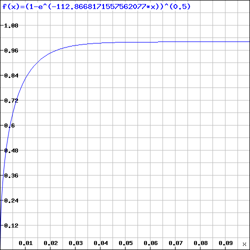
This is a graph of time dilation \(\gamma(x)\) = (1-e^(-112.866*x))^(0.5) around a black hole. Time returns to normal very quickly at about 0.065 m. So much for time travel around a black hole; a 6.5 cm disk around which time dilation occurs is way smaller than expected.
\(g=-\cfrac{{G}_{o}}{(x+{r}_{eo})^2}\)
\({g}_{eo}=-\cfrac{{G}_{o}}{{r}_{eo}^2}\) = -5.07071e18 ms-2
And the corresponding gravity equation is,
\(g=-{g}_{eo}{e}^{-\cfrac{{g}_{eo}{r}_{eo}}{{G}_{o}}(x)}\)
The corresponding time dilation field equation \(\gamma(x)\) is,
\(\gamma(x)=\sqrt{1-\cfrac{2{G}_{o}}{{c}^{2}{r}_{eo}}{e}^{-\cfrac{{g}_{eo}{r}_{eo}}{{G}_{o}}(x)}}\)
\(\cfrac{2{G}_{o}}{{c}^{2}{r}_{eo}}=1\)
\(\cfrac{{g}_{eo}{r}_{eo}}{{G}_{o}}=\cfrac{1}{{r}_{eo}}\) = 112.86681715575618 m-1
\(\gamma(x)=\sqrt{1-e^{-112.866x}}\)
This is a graph of time dilation \(\gamma(x)\) = (1-e^(-112.866*x))^(0.5) around a black hole. Time returns to normal very quickly at about 0.065 m. So much for time travel around a black hole; a 6.5 cm disk around which time dilation occurs is way smaller than expected.
Time Dilation \(\gamma(x)\) around Earth
We know that
\({g}_{o}\) = 9.80663 ms-2, \({r}_{e}\) = 6371000 m
\({G}_{o}\) = 3.980484e14, \(\cfrac{{g}_{o}{r}_{e}}{{G}_{o}}\) = 1.56961e−7
\(g=-{g}_{o}{e}^{-\cfrac{{g}_{o}{r}_{e}}{{G}_{o}}(x)}\)
\(g=-{g}_{o}{e}^{-\cfrac{1}{{r}_{e}}(x)}\)
\(g\) = -9.80665*e^((-1.56961e−7)*x)
And so,
\(\gamma(x)=\sqrt{1-\cfrac{2{G}_{o}}{{c}^{2}{r}_{e}}{e}^{-\cfrac{{g}_{o}{r}_{e}}{{G}_{o}}(x)}}\)
\(\gamma(x)=\sqrt{1-1.3903267*10^{-9}{e}^{-1.56961*{10}^{−7}}(x)}\)
The following show \(\gamma(x)\) with \(x\) scaled by 1000.

As far living on earth is concern, time dilation is very small and it changes very little with the corresponding decrease in gravity as we move away from the gravitational field.
Time Dilation \(\gamma(x)\)
Since,
\(g=-\cfrac { 1 }{ 2 } .\cfrac { d{ v }_{ t }^{ 2 } }{ dx }\)
and
\(\cfrac{{v}_{t}^{2}}{{c}^{2}}=\gamma(x)^{2}\)
\(g=-\cfrac {{c}^{2} }{ 2 } \cfrac { d\gamma(x)^{ 2 } }{ dx }\)
because gravity is given by,
\(g=-{g}_{o}{e}^{-\cfrac{{g}_{o}{r}_{e}}{{G}_{o}}(x)}\)
We have an expression for time dilation \(\gamma\),
\( \cfrac { d\gamma(x)^{ 2 } }{ dx }=\cfrac{2{g}_{o}}{{c}^{2}}{e}^{-\cfrac{{g}_{o}{r}_{e}}{{G}_{o}}(x)}\)
\(\gamma(x)^{ 2 }=\int {d \gamma(x)^{ 2 }}=\int{\cfrac{2{g}_{o}}{{c}^{2}}{e}^{-\cfrac{{g}_{o}{r}_{e}}{{G}_{o}}(x)}dx}\)
\(\gamma(x)^{ 2 }=A-\cfrac{2{G}_{o}}{{c}^{2}{r}_{e}}{e}^{-\cfrac{{g}_{o}{r}_{e}}{{G}_{o}}(x)}\)
When \(x\rightarrow\infty\), \(\gamma(x)^2\rightarrow1\), because \({v}_{t}=c\) when space is normal.
\(\gamma(x)^{ 2 }=1-\cfrac{2{G}_{o}}{{c}^{2}{r}_{e}}{e}^{-\cfrac{{g}_{o}{r}_{e}}{{G}_{o}}(x)}\)
As such a gamma field, the change in \(\gamma=\cfrac{{v}_{t}}{c}\) over \(x\) is given by
\(\gamma(x)=\sqrt{1-\cfrac{2{G}_{o}}{{c}^{2}{r}_{e}}{e}^{-\cfrac{{g}_{o}{r}_{e}}{{G}_{o}}(x)}}\)
This is an expression for time dilation over a gravitational field.
Gravitational Potential Energy
Another way to look at the time dilation equation
\({ v }_{ t }^{ 2 }={c}^{2}-{\cfrac{2{G}_{o}}{{r}_{e}}}{e}^{-\cfrac{{g}_{o}{r}_{e}}{{G}_{o}}(x)}\)
is to see that \(\cfrac{1}{2}{ v }_{ t}^{ 2 }\) is kinetic energy per unit mass. On entering a gravitational field, part of its total energy across space and time dimensions is converted to the term,
\({\cfrac{2{G}_{o}}{{r}_{e}}}{e}^{-\cfrac{{g}_{o}{r}_{e}}{{G}_{o}}(x)}\)
If we compared time dilation equation to
\(\cfrac{1}{2}{ v }_{ t }^{ 2 }+\cfrac{1}{2}{ v }_{ s}^{ 2 }=\cfrac{1}{2}{c}^{2}\)
Then,
\(\cfrac{1}{2}{ v }_{ s}^{ 2 }={\cfrac{{G}_{o}}{{r}_{e}}}{e}^{-\cfrac{{g}_{o}{r}_{e}}{{G}_{o}}(x)}\)
\(|P.E|={\cfrac{{G}_{o}}{{r}_{e}}}{e}^{-\cfrac{{g}_{o}{r}_{e}}{{G}_{o}}(x)}={{g}_{o}{r}_{e}}{e}^{-\cfrac{1}{{r}_{e}}(x)}\) ----(*)
Traditionally we called expression (*) the Gravitational Potential Energy (per unit mass). It is actually energy converted from the total energy of a body in free space to Kinetic Energy in the space dimension, as it enters a gravitational field. GPE is a 'loss' from the total energy, so has a negative value, the body however gain an equivalent amount of Kinetic Energy. The velocity so developed is in the direction of gravity, towards denser space. Loss as GPE is zero where x is far away at infinity where KE is zero also. The odd thing was, why such a conversion from GPE to KE even occurs. The answer is denser space. A gravitational field is just a region of compressed space.
Thursday, April 24, 2014
Time, Time Speed, Aging
If we look at the expression for gravity
\(g=-\cfrac { 1 }{ 2 } .\cfrac { d{ v }_{ t }^{ 2 } }{ dx }\)
Integrating both
\(-2\int { { g } } dx=\int { d{ v }_{ t1 }^{ 2 } } ={ v }_{ t1 }^{ 2 }\)
The left hand side is negative given that g decreases with increasing x.
We have seen that g is of the form, \(g=-{g}_{o}{e}^{-\cfrac{{g}_{o}{r}_{e}}{{G}_{o}}(x)}\), therefore
\(\int { { g } } dx=\cfrac{{G}_{o}}{{r}_{e}}{e}^{-\cfrac{{g}_{o}{r}_{e}}{{G}_{o}}(x)}+A\)
And,
\({ v }_{ t1 }^{ 2 }=C-{\cfrac{2{G}_{o}}{{r}_{e}}}{e}^{-\cfrac{{g}_{o}{r}_{e}}{{G}_{o}}(x)}\)
Since, \({ v }_{ t1 }^{ 2 }={c}^{2}\) when \(x\rightarrow\infty\), where \({d}_{s} \)is at normal space density. \(C={c}^{2}\) and so,
\({v}_{t}=\sqrt{{c}^{2}-{\cfrac{2{G}_{o}}{{r}_{e}}}{e}^{-\cfrac{{g}_{o}{r}_{e}}{{G}_{o}}(x)}}\)
We have an expression similar to before except \(\cfrac{1}{(x+{r}{e})^2}\) is replaced with \({e}^{-\cfrac{{g}_{o}{r}_{e}}{{G}_{o}}(x)}\).
Similarly, time dilation \(\gamma\),
\(\cfrac{{v}_{t}}{c}=\gamma=\sqrt{1-{\cfrac{2{G}_{o}}{{c}^{2}{r}_{e}}}{e}^{-\cfrac{{g}_{o}{r}_{e}}{{G}_{o}}(x)}}\)
In a gravity field time speed is less than time speed at normal space density, \(c\). We experience a shorter second and so, age faster than when gravity is zero where time speed is higher. At higher time speed very second is longer than at slower time speed, if 10 seconds at lower time speed fit into 9 seconds in higher time speed then those at slower time speed is aging 10% faster. Most will think the opposite, that higher time speed mean "time flies" and so age faster or that a second is used up faster. Higher time speed produces a longer second based on a standard second at some standard time speed. A lower time speed travels a shorter second. In the same standard time frame, there are more "short time speed" seconds than "high speed time" seconds. Those at high time speed age less.

Imagine Time has markers make out in space, as space stretches out the time markers stretches out too. X per second means X marks one second. It is confusing because X is also measured in seconds. Time speed should be measured based on some standard time interval for a second, and so X has to be adjusted by a factor inversely proportional its time speed, when taking physics measurements across different time speeds.
Do not be confused by slow-motion cinematic effects, at different time speeds, all will experience time in the same way, within that time speed.
All physics have common expressions across all time speeds within that time speed. The factor, \({\cfrac{{c}}{{v}_{t}}}\) adjustment is needed only when one has to define a standard time interval at speed c, in order to discuss across different time speeds.
\(g=-\cfrac { 1 }{ 2 } .\cfrac { d{ v }_{ t }^{ 2 } }{ dx }\)
Integrating both
\(-2\int { { g } } dx=\int { d{ v }_{ t1 }^{ 2 } } ={ v }_{ t1 }^{ 2 }\)
The left hand side is negative given that g decreases with increasing x.
We have seen that g is of the form, \(g=-{g}_{o}{e}^{-\cfrac{{g}_{o}{r}_{e}}{{G}_{o}}(x)}\), therefore
\(\int { { g } } dx=\cfrac{{G}_{o}}{{r}_{e}}{e}^{-\cfrac{{g}_{o}{r}_{e}}{{G}_{o}}(x)}+A\)
And,
\({ v }_{ t1 }^{ 2 }=C-{\cfrac{2{G}_{o}}{{r}_{e}}}{e}^{-\cfrac{{g}_{o}{r}_{e}}{{G}_{o}}(x)}\)
Since, \({ v }_{ t1 }^{ 2 }={c}^{2}\) when \(x\rightarrow\infty\), where \({d}_{s} \)is at normal space density. \(C={c}^{2}\) and so,
\({v}_{t}=\sqrt{{c}^{2}-{\cfrac{2{G}_{o}}{{r}_{e}}}{e}^{-\cfrac{{g}_{o}{r}_{e}}{{G}_{o}}(x)}}\)
We have an expression similar to before except \(\cfrac{1}{(x+{r}{e})^2}\) is replaced with \({e}^{-\cfrac{{g}_{o}{r}_{e}}{{G}_{o}}(x)}\).
Similarly, time dilation \(\gamma\),
\(\cfrac{{v}_{t}}{c}=\gamma=\sqrt{1-{\cfrac{2{G}_{o}}{{c}^{2}{r}_{e}}}{e}^{-\cfrac{{g}_{o}{r}_{e}}{{G}_{o}}(x)}}\)
In a gravity field time speed is less than time speed at normal space density, \(c\). We experience a shorter second and so, age faster than when gravity is zero where time speed is higher. At higher time speed very second is longer than at slower time speed, if 10 seconds at lower time speed fit into 9 seconds in higher time speed then those at slower time speed is aging 10% faster. Most will think the opposite, that higher time speed mean "time flies" and so age faster or that a second is used up faster. Higher time speed produces a longer second based on a standard second at some standard time speed. A lower time speed travels a shorter second. In the same standard time frame, there are more "short time speed" seconds than "high speed time" seconds. Those at high time speed age less.
All physics have common expressions across all time speeds within that time speed. The factor, \({\cfrac{{c}}{{v}_{t}}}\) adjustment is needed only when one has to define a standard time interval at speed c, in order to discuss across different time speeds.
Graph of Gravity Exponential Form
We know that
\({g}_{o}\) = 9.80663 ms-2, \({r}_{e}\) = 6371000 m
\({G}_{o}\) = 3.980484e14, \(\cfrac{{g}_{o}{r}_{e}}{{G}_{o}}\) = 1.56961e−7
\(g=-{g}_{o}{e}^{-\cfrac{{g}_{o}{r}_{e}}{{G}_{o}}(x)}\)
\(g=-{g}_{o}{e}^{-\cfrac{1}{{r}_{e}}(x)}\)
\(g\) = -9.80665*e^((-1.56961e−7)*x)
The graph below compare the above equations with \(g = -\cfrac{{G}_{o}}{{(x+6371000)}^{2}}\)

Nice, very nice. Here's a scale by 1000 on the x-axis version.

Very nice indeed.
\({g}_{o}\) = 9.80663 ms-2, \({r}_{e}\) = 6371000 m
\({G}_{o}\) = 3.980484e14, \(\cfrac{{g}_{o}{r}_{e}}{{G}_{o}}\) = 1.56961e−7
\(g=-{g}_{o}{e}^{-\cfrac{{g}_{o}{r}_{e}}{{G}_{o}}(x)}\)
\(g=-{g}_{o}{e}^{-\cfrac{1}{{r}_{e}}(x)}\)
\(g\) = -9.80665*e^((-1.56961e−7)*x)
The graph below compare the above equations with \(g = -\cfrac{{G}_{o}}{{(x+6371000)}^{2}}\)
Nice, very nice. Here's a scale by 1000 on the x-axis version.
Very nice indeed.
Gravity Exponential Form
Consider s space density function of the form,
\({ d }_{ s }(x)=A{ e }^{ -bx }+B\) where A, B and b are constant to be determined.
At \({ d }_{ s }(0)={ d }_{ e }\) space is compressed, its space density is \({d}_{s}\), on surface of earth. And \({ d }_{ s }(x\rightarrow \infty )={ d }_{ n }\) where at long distance, space is relaxed and the corresponding space density is \({d}_{n}\).
We have,
\({ d }_{ s }(x)={ e }^{ -bx }({ d }_{ e }{ -d }_{ n })+{ d }_{ n }\) ----(1)
Then we let the inverse relationship between time speed squared \({v}^{2}_{t}\)and space density, \({ d }_{ s }(x)\) to be,
\({v}_{t}^{2}=C-D{ d }_{ s }(x)\) where \(C, D\) are to be determined.
We know that as \(x\rightarrow \infty, { d }_{ s }(x)\rightarrow{ d }_{ n }\)where space is relaxed and time speed is \(c\),
\({v}_{t}^{2}={c}^{2}\), \({ d }_{ s }(x)={ d }_{ n }\)
\(C={c}^{2}+D{d}_{n}\) then,
\({v}_{t}^{2}={c}^{2}-D({ d }_{ s }(x)-{d}_{n})\)
If we then consider the time dilation equation from previously, (The use of this equation is still valid because a linear approach can be consider as a first approximate to an exponential one. Consider the power series expansion of \(e\).)
\({ v }_{ t }= \sqrt {{ c }^{ 2 }-\cfrac { 2{ G }_{ o } }{ (x+r_{ e }) }}\)
when \(x=0\)
\({ v }^{2}_{ t }={ c }^{ 2 }-\cfrac { 2{ G }_{ o } }{ (r_{ e }) }\)
\({v}_{t}^{2}={c}^{2}-D({ d }_{ e } -{d}_{n})\) where \({ d }_{ s }(0)={ d }_{ e }\)
we have,
\(\cfrac { 2{ G }_{ o } }{ (r_{ e })}=D({ d }_{ e } -{d}_{n})\)
therefore,
\(D=\cfrac{ 2{ G }_{ o } }{r_{ e }({ d }_{ e } -{d}_{n})}\)
Hence,
\({v}_{t}^{2}={c}^{2}-\cfrac{ 2{ G }_{ o }({ d }_{ s }(x)-{d}_{n}) }{r_{ e }({ d }_{ e } -{d}_{n})}\)
Differentiating both side with respect to time
\(2{v}_{t}\cfrac{d{v}_{t}}{dt}=-\cfrac{2{G}_{o}}{{r}_{e}({d}{e}-{d}{n})}\cfrac{d({d}_{s}(x))}{dx}\cfrac{dx}{dt}\)
\({v}_{t}\cfrac{d{v}_{t}}{dt}=-\cfrac{{G}_{o}}{{r}_{e}({d}{e}-{d}{n})}\cfrac{d({d}_{s}(x))}{dx}{v}_{s}\) ----(2)
But from the energy equation,
\({v}^{2}_{t}+{v}^{2}_{s}={c}^{2}\) differentiating it
\(2{v}_{t}\cfrac{d{v}_{t}}{dt} + 2{v}_{s}\cfrac{d{v}_{s}}{dt}=0\), since \(\cfrac{d{v}_{s}}{dt}=g\)
\(2{v}_{t}\cfrac{d{v}_{t}}{dt} = -2g.{v}_{s}\)
\(g.{v}_{s}=-{v}_{t}\cfrac{d{v}_{t}}{dx}\) substitute into (2)
and so,
\(g=\cfrac{{G}_{o}}{{r}_{e}({d}_{e}-{d}_{n})}.\cfrac{d({d}_{s}(x))}{dx}\)
From (1), differentiating with respect to x,
\(\cfrac{d({d}_{s}(x))}{dx}=-b{e}^{-b(x)}({d}_{e}-{d}_{n})\) subsitute into the above we have,
\(g=\cfrac{{G}{o}}{{r}_{e}}.(-b).{e}^{-b(x)}\)
But we know that at \(x=0\),
\(g={g}_{o}=-b\cfrac{{G}_{o}}{{r}_{e}}\), therefore,
\(b=\cfrac{{g}_{o}{r}_{e}}{{G}_{o}}=\cfrac{1}{{r}_{e}}\) \(\because {g}_{o}=\cfrac{{G}_{o}}{{r}^2_{e}}\)
And so we have an expression for gravity,
\(g=-{g}_{o}{e}^{-\cfrac{{g}_{o}{r}_{e}}{{G}_{o}}(x)}\) the negative sign indicates the direction of g.
This expression is based on compression of free space, in a exponential manner.
Tuesday, April 22, 2014
Linear Approximation to Space Density Compression
Consider
\( { v }_{ t }^{ 2 }=\cfrac { A }{ { d }_{ s } }\) where A is a constant
that shows time speed is inversely proportional to space density. So
\( { c }^{ 2 }=\cfrac { A }{ { d }_{ normal} }\)
ie. \(A={c}^{2}{d}_{normal}\)
with the understanding that at normal space density time \({d}_{normal}\) speed is c. And
\({ d }_{ s }=-a(x+{ r }_{ 0 })+{ a }_{ 0 }\) ----(*)
that gives linear space density change. And
\(g=-\cfrac { 1 }{ 2 } .\cfrac { d{ v }_{ t }^{ 2 } }{ dx } =-\cfrac { 1 }{ 2 } .\cfrac { d }{ dx } (\cfrac { A }{ { d }_{ s } } )=\cfrac { A }{ 2 } .\cfrac { 1 }{ { d }_{ s }^{ 2 } } .\cfrac { d{ d }_{ s } }{ dx }\)
\(g=-G.\cfrac { 1 }{ { (-a(x+{ r }_{ o })+{ a }_{ 0 }) }^{ 2 } } =-\cfrac { G }{ { a }^{ 2 } } \cfrac { 1 }{ { (x+\cfrac { { a{ r }_{ o }-a }_{ o } }{ a } ) }^{ 2 } } =-\cfrac { G }{ { a }^{ 2 } } \cfrac { 1 }{ { (x+{ r }_{ e }) }^{ 2 } }=-{ G }_{ 0 }.\cfrac { 1 }{ { (x+{ r }_{ e }) }^{ 2 } }\)
that expresses gravity derived from considering the energy conservation equation and changing space density affecting time speed. Looking at \({G}_{o}\)
\(G=\cfrac{Aa}{2}\) and so,
\({G}_{o}=\cfrac{G}{{a}^{2}}=\cfrac{A}{2a}\)
Therefore
\(a=\cfrac{{c}^{2}{d}_{normal}}{2{G}_{o}}=\cfrac{{d}_{normal}}{{r}_{eo}}\), since \({r}_{eo}=\cfrac{2{G}_{o}}{{c}^{2}}\)
When \(x=0\) the space density equation gives
\({d}_{s}={d}_{earth}=-\cfrac{{d}_{normal}}{{r}_{eo}}({ r }_{ 0 })+{ a }_{ 0 }\)
so,
\({ a }_{ 0 }={d}_{earth}+\cfrac{{d}_{normal}}{{r}_{eo}}{ r }_{ 0 }\)
and so (*) becomes
\({d}_{s}(x)=-\cfrac{{d}_{normal}}{{r}_{eo}}(x+{ r }_{ 0 })+{d}_{earth}+\cfrac{{d}_{normal}}{{r}_{eo}}{ r }_{ 0 }\)
\({d}_{s}(x)=-\cfrac{{d}_{normal}}{{r}_{eo}}(x)+{d}_{earth}\) or
\({d}_{s}(x)=-\cfrac{{c}^{2}{d}_{normal}}{2{G}_{o}}(x)+{d}_{earth}\)
We see clearly the absurdity of this formulation but as a first linear approximation it is OK. The factor
\(\cfrac { 1 }{ { d }_{ s }^{ 2 } } .\cfrac { d{ d }_{ s } }{ dx }\)
needs further consideration, in order that the space density equation make more sense. Consider, the expansion.
\({e}^{-b(x+{r}_{e})}={e}^{-b{r}_{e}}(1-bx+.....)=(-{e}^{-b{r}_{e}}bx+{e}^{-b{r}_{e}}....).\)
then \({d}_{s}(x)={e}^{-b(x)}{e}^{-b{r}_{e}}\), where \({e}^{-b{r}_{e}}={d}_{earth}\), \( b=\cfrac { { c }^{ 2 }{ d }_{ normal } }{ 2{ G }_{ o }{d}_{earth} }\) and \({ e }^{ -\cfrac { { c }^{ 2 }{ d }_{ normal } }{ 2{ G }_{ o }{d}_{earth} } { r }_{ e } }={ d }_{ earth }\)
where \(a, b\) are constants and \({r}_{e}\) is defined such that x=0 is on the surface of earth where space is most compressed. By comparing coefficients, we have a consistent expression,
\({ d }_{ s }(x)={ e }^{ -\cfrac { { c }^{ 2 }{ d }_{ normal } }{ 2{ G }_{ o }{d}_{earth}} (x) }{ e }^{ -\cfrac { { c }^{ 2 }{ d }_{ normal } }{ 2{ G }_{ o }{d}_{earth} } { r }_{ e } }+{d}_{normal}\)
The last term is added because we know that \(x\rightarrow \infty \), \({d}_{s}\rightarrow{d}_{normal}\) and the term constant term \(e^{-b{r}_{e}}\) is modified to
\({ e }^{ -\cfrac { { c }^{ 2 }{ d }_{ normal } }{ 2{ G }_{ o }{d}_{earth} } { r }_{ e } }={ d }_{ earth }-{d}_{normal}\).
\({ d }_{ s }(x)={ e }^{ -\cfrac { { c }^{ 2 }{ d }_{ normal } }{ 2{ G }_{ o }{d}_{earth}} (x) }({ d }_{ earth }-{d}_{normal})+{d}_{normal}\)
This derivation however, will lead to unfamiliar expressions, although we have seen the first approximation to be the same as textbook derivation. Have a nice day.
No Prime \(E[{N}_{x}]\)
Consider again,
\({\prod _{ 1 }^{ { N }_{ x }}{ (\frac { 1 }{ 2 } )(\frac { 2 }{ 3 } )(\frac { 4 }{ 5 } )(\frac { 6 }{ 7 } )...\frac{{P}_{N}-1}{{P}_{N}}}}\)
This term can be evaluated for all \({N}_{x}\) but the summation of its product with \({N}_{x}\) is not. It is possible to evaluate \(E[{N}_{x}]\) for a bounded set but not for all primes. The proof that there are infinite numbers of primes suggests that the tail of the Probability \({N}_{x}\)of being Prime graph is never zero. And as \({N}_{x}\) tends towards infinity, the term
\(\frac{{N}_{x}-1}{{N}_{x}}=1-\frac{1}{{N}_{x}}\) is divergent with respect to \(\int { (1-\frac { 1 }{ { N }_{ x } } ) } d{ N }_{ x }\).
Monday, April 21, 2014
Black Hole Mass Density
From previously, if earth were to shrink to a radius of \({r}_{o}=0.00886\)m then it is dense enough to be a black hole. Since,
\(\cfrac { { r }_{ e }^{ 3 } }{ { r }_{ o }^{ 3 } } =\cfrac { { d }_{ o } }{ { d }_{ e } }\) , earth density, \({d}_{e}\) = 5.52 g/cm³, earth radius, \({r}_{e}\)=6371 km
We have mass density of this black hole, \({d}_{o}\)
\({ d }_{ o }=\cfrac { { r }_{ e }^{ 3 } }{ { r }_{ o }^{ 3 } } { d }_{ e }\)=(6371000/0.00886)^3*5.52= 2.0524*10^27 g/cm³
Space permeates through all matter. This density may be the limit beyond which space cannot penetrate.
Moving Space
The existence of Casimir Effect suggests that there cannot be arbitrarily small volume of space. Imagine constructing a box of length less than the gap dimension between Casimir parallel plates. Such a box will collapse onto itself. One can then imagine, the whole universe as being made of up such cubes of Casimir Effects dimension and no smaller.
X out of Y and X out of Y
Why would the probabilities of being prime be an indication of the distribution of numbers around primes? If \({N}_{x}\) has a probability of \(\frac{x}{y}\) of being a prime, that means out of y numbers x are prime around that locality where \({N}_{x}\) is. Conversely, such probabilities are also good indications of the distribution of primes, for x out of y numbers are prime, around the same area.
I am not sure what Riemann and Euler did to prime numbers, but it seems overtly complicated and a pole at s=1 is ugly, especially if you don't think it effects the numbers around it by taking limits and assigning finite values to s, the complex variable.
I am not sure what Riemann and Euler did to prime numbers, but it seems overtly complicated and a pole at s=1 is ugly, especially if you don't think it effects the numbers around it by taking limits and assigning finite values to s, the complex variable.
Sunday, April 20, 2014
Prime Probability Curve
A graph of this probability
\(P({N}_{x})=\prod _{ i=1 }^{ { P }_{ N }<{ N }_{ x }<{ P }_{ N+1 } }{ \frac { { P }_{ i }-1 }{ { P }_{ i } } } \), when \({ P }_{ N }={ N }_{ x }\) the associated probability is 1.
as \({N}_{x}\) increases leaving out all prime numbers is a good indication of the distribution of numbers around the primes. The probability graph of \({N}_{x}\) seemed to have an asymptote at around \(P({N}_{x}\))=0.0412 for \({N}_{x}\) large.

This graph was generated from a list of primes up to and including 821641. The initial sharp drop down the y-axis is due to new discoveries of small primes that rule out many higher numbers as candidate for primes. The graph seem to have an asymptote, but is actually decreasing very slowly. There are simply not enough small numbers to go around, especially small prime numbers. This then is the distribution of primes.
Prime Probability
The probability that \({N}_{x}\) is a prime is given by
\(\prod _{ i=1 }^{ { P }_{ N }<{ N }_{ x }<{ P }_{ N+1 } }{ \frac { { P }_{ i }-1 }{ { P }_{ i }}=\prod _{ i }^{ { P }_{ N } }{ (1-\frac { 1 }{ { P }_{ i } }) }} \) when \({ P }_{ N }={ N }_{ x }\) the associated probability is 1.
where \( { P }_{ N }\) is the \(Nth\) prime smaller but closest to or equal to \({ N }_{ x }\).
The expected value of \({ N }_{ x }\) statistically is then,
\(E\left[ { N }_{ x } \right] =\sum _{ 1 }^{ x\rightarrow \infty }{ ({ N }_{ x } \prod _{ i=1 }^{ { P }_{ N }<{ N }_{ x }<{ P }_{ N+1 } }{ \frac { { P }_{ i }-1 }{ { P }_{ i } } } } )\)
the summation is over all \({N}_{x}\) positive integer; and 1 not being a prime by definition.
\(E\left[ { N }_{ x } \right] =\sum _{ 2 }^{ x\rightarrow \infty }{ ({ N }_{ x } \prod _{ i=1 }^{ { P }_{ N }<{ N }_{ x }<{ P }_{ N+1 } }{ \frac { { P }_{ i }-1 }{ { P }_{ i } } } } )\)
The starting value of 1 prove to be very troublesome as far as consistency is concern. The value of \(\frac{1}{2}\) for \({P}_{2}\) can be argued as the probability of any number \({N}_{x}\) being odd or even. Strictly speaking \(2≮2\) and so \(?<2<2\) from the expression \({ P }_{ N }<{ N }_{ x }<{ P }_{ N+1 }\) does not hold.
Consider the term \( { P }_{ N }<{ N }_{ x }<{ P }_{ N+1 }\) , the numbers \({N}_{x}\) between
two consecutive primes \( { P }_{ N }, { P }_{ N+1 }\). All these numbers will share the same probability of
\({\prod _{ 1 }^{ { N }_{ x } }{ (\frac { 1 }{ 2 } )(\frac { 2 }{ 3 } )(\frac { 4 }{ 5 } )(\frac { 6 }{ 7 } )...\frac{{P}_{N}-1}{{P}_{N}}}}\)
Some may argue that since such \({N}_{x}\) are between two consecutive primes, they are not primes and so have a probability of zero being prime. The point is to calculate expected value \(E[{N}_{x}]\); \({N}_{x}\) is considered a random variable here. The expected value of \({N}_{x}\) being prime is not the average value of primes in a given set of prime numbers.
Probability of Being Prime
With prime number it is very easy to get caught up with to much algebra and complex numbers. A very basic simplification is to realize that prime numbers that occurred become factors to exclude many numbers as possible candidate as prime numbers. 2 for example reduces all likely prime numbers to be odd only. So, walking along odd number line \(n\) is replaced with \(2n+1\).
odd \(3n\) becomes \(6n+3\) with 2 odd numbers between consecutive odd multiples of 3
odd \(5n\) becomes \(10n+5\) with 4 odd numbers between consecutive odd multiples of 5
odd \(7n\) becomes \(14n+7\) with 6 odd numbers between consecutive odd multiples of 7
odd \(11n\) becomes \(22n+11\) with 10 odd numbers between consecutive odd multiples of 11
So, given a odd number \({N}_{x}\) just greater that 11, the next lower prime. We have,
2/3 = probability that \({N}_{x}\) is not a multiple of 3
4/5 = probability that \({N}_{x}\) is not a multiple of 5
6/7 = probability that \({N}_{x}\) is not a multiple of 7
10/11 = probability that \({N}_{x}\) is not a multiple of 11
and so the probability that \({N}_{x}\) is a prime is
\(\prod _{ i }^{ { P }_{ N }<{ N }_{ x }<{ P }_{ N+1 } }{ \frac { { P }_{ i }-1 }{ { P }_{ i } } } \) when \({ P }_{ N }={ N }_{ x }\) the associated probability is 1.
In general, any number being prime is given by the above expression where \(i=1\), \({P}_{1}=2 \) is the first prime.
What is really interesting is as \({ N }_{ x }\rightarrow \infty \)
\({ \prod _{ 1 }^{ { N }_{ x }\rightarrow \infty }{ (\frac { 1 }{ 2 } )(\frac { 2 }{ 3 } )(\frac { 4 }{ 5 } )(\frac { 6 }{ 7 } )...\quad ({ P }_{ i }<1)... } }=0\).
That is to say, given any number, big enough, it is not likely to be a prime number. For example, any number \(99991<{N}_{x}<100003\) has the probability of 0.048752917851015 of being a prime. And any number \(821603<{N}_{x}<821641\) has the probability of 0.0412229294373678 of being a prime. Not bad 4% chance. This probability deceases as \({N}_{x}\) increases. Infinity is not likely a prime.
Friday, April 18, 2014
Tuesday, April 15, 2014
Fermat's Last Theorem, here's a broader margin.
So, about Fermat's Last Theorem where a,b,c are integers
\({ a }^{ n }+{ b }^{ n }={ c }^{ n }\quad Let\quad x+1=a,\quad y+1=b,\quad z=c,\) so \(a,b>1\)
We have
\({ \left( x+1 \right)}^{ n }+{ \left( y+1 \right)}^{ n }-{ z }^{ n }=0\)
Consider
\({ \left[ \left( x+1 \right) +\left( y+1 \right)\right]}^{ n }=\quad { \left( x+1 \right)}^{ n }+{ \left( y+1 \right)}^{ n }\\ \quad \quad \quad \quad \quad \quad \quad \quad \quad +\left( \begin{matrix} n \\ 1 \end{matrix} \right) \left( x+1 \right) { \left( y+1 \right)}^{ n-1 }\\\quad \quad \quad \quad \quad \quad \quad \quad \quad +\left( \begin{matrix} n \\ 2 \end{matrix} \right) { \left( x+1 \right)}^{ 2 }{ \left( y+1 \right)}^{ n-1 }\\ \quad \quad \quad \quad \quad \quad \quad \quad \quad +...\\\quad \quad \quad \quad \quad \quad \quad \quad \quad +\left( \begin{matrix} n \\ n-1 \end{matrix} \right) { \left( x+1 \right)}^{ n-1 }{ \left( y+1 \right)}^{ 1 }\)
then
\({ \left[ \left( x+1 \right) +\left( y+1 \right)\right]}^{ n }-{ z }^{ n }>{\left( x+1 \right)}^{ n }+{ \left( y+1 \right)}^{ n }-{ z }^{ n }\)
Also,
\({ \left( x+1 \right)}^{ n }={ x }^{ n }+\left( \begin{matrix} n \\ 1 \end{matrix} \right) { x }^{ n-1 }+\left( \begin{matrix} n \\ 2 \end{matrix} \right) { x }^{ n-2 }+...+\left( \begin{matrix} n \\ n-1 \end{matrix} \right) x+1\\ { \left( y+1 \right)}^{ n }=y^{ n }+\left( \begin{matrix} n \\ 1 \end{matrix} \right) y^{ n-1 }+\left( \begin{matrix} n \\ 2 \end{matrix} \right) { y }^{ n-2 }+...+\left( \begin{matrix} n \\ n-1 \end{matrix} \right) y+1\\ { \left( z+1 \right) }^{ n }=z^{ n }+\left( \begin{matrix} n \\ 1 \end{matrix} \right) z^{ n-1 }+\left( \begin{matrix} n \\ 2 \end{matrix} \right) { z }^{ n-2 }+...+\left( \begin{matrix} n \\ n-1 \end{matrix} \right) z+1\)
We have,
\({ \left[ \left( x+1 \right) +\left( y+1 \right)\right]}^{ n }-{ z }^{ n }=\quad { x }^{ n }+y^{ n }-{ z }^{ n }\\\quad \quad \quad \quad \quad \quad \quad \quad \quad +\left( \begin{matrix} n \\ 1 \end{matrix} \right) \left[ { x }^{ n-1 }+\left( x+1 \right) { \left( y+1 \right)}^{ n-1 }+{ y }^{ n-1 } \right] \\\quad \quad \quad \quad \quad \quad \quad \quad \quad +\left( \begin{matrix} n \\ 2 \end{matrix} \right) \left[ { x }^{ n-2 }+{ \left( x+1 \right)}^{ 2 }{ \left( y+1 \right)}^{ n-2 }+{ y }^{ n-2 } \right] \\ \quad \quad \quad \quad \quad \quad \quad \quad \quad +...\\ \quad \quad \quad \quad \quad \quad \quad \quad \quad +\left( \begin{matrix} n \\ n-1 \end{matrix} \right) \left[ x+{ \left( x+1 \right)}^{ n-1 }\left( y+1 \right) +y \right] \\\quad \quad \quad \quad \quad \quad \quad \quad \quad +2\)
\({ \left[ \left( x+1 \right) +\left( y+1 \right)\right]}^{ n }-{ z }^{ n }=\quad { x }^{ n }+y^{ n }-{ z }^{ n }\\ \quad \quad \quad \quad \quad \quad \quad \quad \quad +\left( \begin{matrix} n \\ 1 \end{matrix} \right) \left[ { x }^{ n-1 }+{ f }_{ 1 }\left( x,y \right) +{ y }^{ n-1 } \right] \\ \quad \quad \quad \quad \quad \quad \quad \quad \quad +\left( \begin{matrix} n \\ 2 \end{matrix} \right) \left[ { x }^{ n-2 }+{ f }_{ 2 }\left( x,y \right) +{ y }^{ n-2 } \right] \\ \quad \quad \quad \quad \quad \quad \quad \quad \quad +...\\ \quad \quad \quad \quad \quad \quad \quad \quad \quad +\left( \begin{matrix} n \\ n-1 \end{matrix} \right) \left[ x+{ f }_{ n-1 }\left( x,y \right) +y \right] \\ \quad \quad \quad \quad \quad \quad \quad \quad \quad +2\\ \quad \quad \quad \quad \quad \quad \quad \quad \quad +\sum _{ i=1 }^{ n-1 }{ \left( \begin{matrix} n \\ i \end{matrix} \right)} \)
then
\({ \left[ \left( x+1 \right) +\left( y+1 \right)\right]}^{ n }-{ z }^{ n }>{ \left( x+1 \right)}^{ n }+{ \left( y+1 \right)}^{ n }-{ z }^{ n }\)
\({ \left( x+1 \right)}^{ n }+{ \left( y+1 \right)}^{ n }-{ z }^{ n }>{ x }^{ n }+{ y }^{ n }-{ z }^{ n }+2+\sum _{ i=1 }^{ n-1 }{ \left( \begin{matrix} n \\ i \end{matrix} \right)} \)-----------(2a)
\({ \left( x+1 \right)}^{ n }+{ \left( y+1 \right)}^{ n }-{ z }^{ n }>{ x }^{ n }+{ y }^{ n }-{ z }^{ n }\) ---------------------------(1)
\({ x }^{ n }+y^{ n }-{ z }^{ n }+2+\sum _{ i=1 }^{ n-1 }{ \left( \begin{matrix} n \\ i \end{matrix} \right)}>{ x }^{ n }+y^{ n }-{ \left( z+1 \right) }^{ n }+2+\sum _{ i=1 }^{ n-1 }{ \left( \begin{matrix} n \\ i \end{matrix} \right)} \) -----------(2b)
and so, when
\({ \left( x+1 \right)}^{ n }+{ \left( y+1 \right)}^{ n }-{ z }^{ n }=0\) -------------(S)
then from expression (2a) and (2b)
\({ x }^{ n }+y^{ n }-{ \left( z+1 \right) }^{ n }+2+\sum _{ i=1 }^{ n-1 }{ \left( \begin{matrix} n \\ i \end{matrix} \right)}<0\)
and from expression (1)
\({ x }^{ n }+{ y }^{ n }-{ z }^{ n }<0\)
that is \({ \left( z+1 \right)}^{ n }-{ z }^{ n }<2+\sum _{ i=1 }^{ n-1 }{ \left( \begin{matrix} n \\ i \end{matrix} \right)}\)
\({ \left( z+1 \right)}^{ n }-{ z }^{ n }=\left( \begin{matrix} n \\ 1 \end{matrix} \right) z^{ n-1 }+\left( \begin{matrix} n \\ 2 \end{matrix} \right) { z }^{ n-2 }+...+\left( \begin{matrix} n \\ n-1 \end{matrix} \right) z+1\)
\(=\sum _{ i=1 }^{ n-1 }{ \left( \begin{matrix} n \\ i \end{matrix} \right)z^{ n-i }+1}<2+\sum _{ i=1 }^{ n-1 }{ \left( \begin{matrix} n \\ i \end{matrix} \right)}\) -------------(3)
for \(n=2\)
\(\left( \begin{matrix} 2 \\ 1 \end{matrix} \right) z+1<\sum _{ 1 }^{ 1 }{ \left( \begin{matrix} 2 \\ i \end{matrix} \right)} \quad 2z<3\) which can be true. (This is a statment that was derived from the starting condition (S) that prove to be possible.)
but for \(n=3\)
\(\left( \begin{matrix} 3 \\ 1 \end{matrix} \right) z^{ 2 }+\left( \begin{matrix} 3 \\ 2 \end{matrix} \right) z+1<2+\sum _{ i=1 }^{ 2 }{ \left( \begin{matrix} 3 \\ i \end{matrix} \right)} \)
\( 3{ z }^{ 2 }+3z\nless7\) for all \(z > 1\).
In fact we have a contradiction for all \(n>2\) because the expression \(\sum _{ i=1 }^{ n-1 }{ \left( \begin{matrix} n \\ i \end{matrix} \right)} \) is just the coefficients of the \(z\) on the L.H.S. of expression (3). (For \(n>2\) the derived statment proved to be false, invalidating the starting condition (S).) And so, \({ \left( x+1 \right)}^{ n }+{ \left( y+1 \right)}^{ n }\neq{ z }^{ n }\) for \(n>2\).
Therefore,
\({ a }^{ n }+{ b }^{ n }={ c }^{ n }\) has no valid solution for \(n>2\) and \(a,b>1\)
And that's Fermat's Last Theorem, proved by contradiction.
(Expression (3) is derived from (S), it is not an attempt to solve for \(z\).)
Monday, April 14, 2014
Conservation across dimensions, Symmetry Only
The conservation of energy across time and space dimension is not new. Under normal circumstances, energy discrepancies as a result of heat, EM radiation, increase in stored energies of all kind, etc have to be accounted for. Total energy across all dimensions must be accounted for. More importantly, all valid dimensions have both kinetic and potential energy terms. Time for example has kinetic energy and it is expected to have potential time energy, an expression for time force and an expression for time momentum. In fact, all dimensions should have similar expressions; physic expressions in one dimension, for example space x, is indistinguishable mathematically from expressions in other valid dimensions.
Sunday, April 13, 2014
Moving in Two Directions at the Same Time
Moving space around also resolve the seeming impossibility of moving in two or more directions at the same time. Moving space upwards relatively means a body is falling downwards, at some point the body will experience free-fall, that is to say, no gravity. Alternatively, space compresses upwards, creating a region of high gravity upwards. This cancels with normal gravity downwards and the body once again experiences weightlessness. Both aspects are equivalent. The point is to move space about.
Over the Head, Complex
What then is this mysterious complex component, \(i{v}_{s}\)?
\({v}_{s}\)\(\nwarrow \nearrow\) \({v}_{t}\)
\(\swarrow \)\(i{v}_{s}^{ ' }\)
The time dimension is always orthogonal to the space dimension. The direction of \({v}_{s}\) is a reference, orthogonal to this direction is the time dimension. The value of \({v}_{s}\) is not that important as far as a directional reference is concerned. One way to generate \(i{v}_{s}^{ ' }\) is to have space rotate about the direction of \({v}_{s}\), perpendicular to \({v}_{s}\). Space moving, is relatively the same as moving through space. This then makes time travel possible. Time travel in both direction, to the future and to the past, as \(i{v}_{s}^{ ' }\) can be made to add to \({v}_{t}\) or substrate from it. Theoretically.
Time Travel is Complex
If we look again at the conservation of energy equation,
\( { v }_{ t }^{ 2 }+{ v }_{ s }^{ 2 }={ c }^{ 2 }\)
what happens when \( { v }_{ s }>{ c }\),
\( { v }_{ t }^{ 2 }= -{ V }^{ 2 }\) where \({ V }^{ 2 }={ v }_{ s }^{ 2 }-{ c }^{ 2 }\)
\( { v }_{ t }^{ ' }=iV\)
\(\nwarrow \quad +\quad \nearrow \quad +\quad \swarrow \quad=\quad \upuparrows \)
\( { v }_{ t }\) \( { v }_{ s }\) \( i{ v }_{ t }^{ ' }\) \( {c }\)
A complex component develops in \({ v }_{ t } \) that cancels that part of \({ v }_{ s }\) that is greater that \({ c }\). The use of \( i{ v }_{ t }^{ ' }\) is to illustrate that \( { v }_{ t }\) and \( i{ v }_{ t }^{ ' }\) are not of the same magnitude.
Similarly, if we develop a complex component in \({ v }_{ s }\) we will then be able to cancel part of \({ v }_{ t } \) and given a great enough complex component in \({ v }_{ s }\), we will be able to make \({ v }_{ t } \) negative. \( { v }_{ t }\), \( { v }_{ s }\) are dummy variables we can swap them and we have
\(\nwarrow \quad +\quad \nearrow \quad +\quad \swarrow \quad=\quad \upuparrows \)
\( { v }_{ s }\) \( { v }_{ t }\) \( i{ v }_{ s }^{ ' }\) \( {c }\)
Remember that \( {c }\) is a constant. If we are able to generate \( i{ v }_{ s }^{ ' }\) we can then slow \( { v }_{ t }\) and even reverse \( { v }_{ t }\).
No Time for Information
The good thing about this derivation is that time stands still in a black hole. A conclusion that preempt a lot of arguments and speculations.
Black Hole
And from the conservation of energy equation,
\( { v }_{ t }^{ 2 }+{ v }_{ s }^{ 2 }={ c }^{ 2 }\)
when \( { v }_{ t }=0\),
\({ v }_{ s }={ c }\)
that means the body falling into such a gravitational field will tend towards light speed.
Conversely, if a body is at rest in such a gravitational field it will have to gain light speed to escape such a field. When,
\({ r }_{ o }<0.00886 m\)
that is to say a denser body, we will need speed greater that light speed to escape, and light itself will not be able to escape from this gravitational field. Yes, we have a black hole.
Thank you for being here.
No Time, No Light, No Escape
Consider the time speed equation,
\({ v }_{ t }= \sqrt {{ c }^{ 2 }-\cfrac { 2{ G }_{ o } }{ (x+r_{ e }) } }\)
Can space be so dense that at \( x=0\) that time speed is zero. That time itself stopped. Theoretically, that can happen when
\( { c }^{ 2 }=\cfrac { 2{ G }_{ o } }{ (r_{ e }) } \)
that is when \({ r }_{ eo }\) is given by the expression
\({ r }_{ eo }=\cfrac { 2{ G }_{ o } }{ { c }^{ 2 } }\) (*)
But first we have to calculate \({ G }_{ o }\). Using earth as an example, where \(g\) = 9.80665 ms-2 on the surface of earth, and \({ r }_{ e }\) = 6371 km, from previously
\(g=-{ G }_{ o }.\cfrac { 1 }{ { (x+{ r }_{ e }) }^{ 2 } }\), \(x=0\)
We have,
\( |g|=\cfrac { { G }_{ o } }{ { r }_{ e }^{ 2 } } \)
\({ G }_{ o }=|g|.{ { r }_{ e }^{ 2 } }\)
\({ G }_{ o }\) = 9.80665*(6.371e6 )^2 = 3.980484e14
With \(c\) = 299792458 ms-2, from equation * when
\({ r }_{ eo }\) = 0.00886 m time speed \({ v }_{ t }\) is zero.
This means that if earth is to be squeezed to a size of 8.86 mm, time would stand still on its surface.
Background = Most Pervasive = Resonnace
This is the resonance of the electromagnetic dipole not of free space
The cosmic microwave background radiation spectrum peaks at 160.2 GHz, corresponding to a wavelength of 1.9 mm. If we model space as light springs, then we can expect this frequency to be the resonance frequency of free space. It is at this frequency that radiation losses are less and so will exhibit as a peak in the spectrum. The resonance frequency formula,
\({ f }_{ res }=\cfrac { 1 }{ 2\pi } \sqrt { \cfrac { k }{ { m } } }\)
is still valid if we redefine m as \({ \Delta m }\) a small mass element of space.
\({ f }_{ res }=\cfrac { 1 }{ 2\pi } \sqrt { \cfrac { k }{ { \Delta m } } }\)
from which we refine to
\({ f }_{ res }=\cfrac { 1 }{ 2\pi } \sqrt { { k }_{ space } }\) and
\({ k }_{ space }={ (2\pi { f }_{ res }) }^{ 2 }\)
where \({ k }_{ space }\) is defined as spring constant per unit mass
\({ k }_{ space }=1.0131757\times { 10 }^{ 24 }{ s }^{ -2 }\)
\(K_space\) is still valid but it is of the dipole that carries electromagnetic waves.
Saturday, April 12, 2014
Orthogonal Dimensions
The time dimension and space dimension is orthogonal. A change in the time dimension should have no effect in the space dimension and vice versa. A force changing space velocity has no direct effect on time velocity. However, a body moving through space, is relatively the same as having space move through the body. As such a moving body experiences time differently.
Friday, April 11, 2014
Initial Kick at Warp Speed
Notice that time dilation \(\gamma \) is independent of \({ v }_{ s }\), this means a body experiences time dilation because of a change in gravity only, irrespective of its space velocity. However, as a body increased speed, the relative space density in the direction of its travel increases. The situation is analogous to a body at rest counting a number of smaller bodies around it per unit volume. If at speed v the body counts A then at speed 2v it will count 2A. The relative space density increases proportionally with its space velocity.
Consider the expression
\({ v }_{ s }tA{ d }_{ s }\), for time t, unit area A, where \({ v }_{ s }\) is space velocity and \({ d }_{ s }\) space density.
at speed \(B{ v }_{ s }\) we have \(B{ v }_{ s }tA{ d }_{ s }\) which is \({ v }_{ s }tA(B{ d }_{ s })\) which suggest a relative increase in space density
This leads us to,
\(\cfrac { { v }_{ s1 } }{ { v }_{ s2 } } =\cfrac { { d }_{ s1 } }{ { d }_{ s2 } }\)
but
\({ v }_{ t }^{ 2 }\propto \cfrac { 1 }{ { d }_{ s } }\)
as such
\(\cfrac { { v }_{ t1 }^{ 2 } }{ { v }_{ t2 }^{ 2 } } =\cfrac { { d }_{ s2 } }{ { d }_{ s1 } } =\cfrac { { v }_{ s2 } }{ { v }_{ s1 } }\)
which gives us
\({ v }_{ t1 }={ v }_{ t2 }\sqrt { \cfrac { { v }_{ s2 } }{ { v }_{ s1 } } }\)
This result is without any experimental proof! And is actually running away. In reality space does not pile up indefinitely in front of the moving body. Space like a light fluid, flows around the body as the body moves through it. However, an initial increase in space velocity causes time velocity to decrease resulting in a further increase in space velocity (via, \( { v }_{ t }^{ 2 }+{ v }_{ s }^{ 2 }={ c }^{ 2 }\) ) . An initial kick in the rear, nothing more.
What about \(\gamma(x)\)?
The expression for time speed
\({ v }_{ t }= \sqrt {{ c }^{ 2 }-\cfrac { 2{ G }_{ o } }{ (x+r_{ e }) } }\)
is in the time domain. Whereas x is measured from dense space to less dense space. This velocity when multiplied by \({ t }_{ c }\) the standard time when time speed \({ v }_{ c }=c\) gives the duration of a second as experienced by a body at distance x. Dividing by normal time speed c, we have an expression for time dilation.
\(\gamma =\cfrac { { v }_{ t } }{ c } =\sqrt { 1-\cfrac { 2{ G }_{ o } }{ { c }^{ 2 }(x+r_{ e }) } } \)
As we move away from a gravitational field, time returns to normal time speed. Inside the influence of gravity, compressed space, time speed is lower, as such time dilates when we leave the gravitational field and time speed increases.
This is time dilation. Dividing distance in the space dimension by space velocity does not give you distance in standard seconds in the time dimension. We experience time along the time dimension.
At distance far away from the influence of gravity, time is normal at time speed c, therefore \(\gamma \le 1\).
Time Speed Field
If we look at the expression for gravity
\(g=-\cfrac { 1 }{ 2 } .\cfrac { d{ v }_{ t }^{ 2 } }{ dx }\)
Integrating both sides
\(-2\int { { g } } dx=\int { d{ v }_{ t1 }^{ 2 } } ={ v }_{ t1 }^{ 2 }\) ----(1)
The left hand side is negative given that g decreases with increasing x.
We have seen that g is of the form,
\(g=-{ G }_{ o }.\cfrac { 1 }{ { (x+{ r }_{ e }) }^{ 2 } }\)
where the negative sign suggests that g, a vector is pointing towards x=0. Integrating,
\(\int { g } dx={ G }_{ o }.\cfrac { 1 }{ (x+{ r }_{ e }) }+A\) ----(2)
Combining the above equations (1) and (2) and using constant C=-2A
\({ v }_{ t }= \sqrt { C-\cfrac { 2{ G }_{ o } }{ (x+r_{ e }) } }\)
Since we know that at no gravity, space is not compressed where \(x\rightarrow \infty \), \({ v }_{ t }=c\), we have \(C={ c }^{ 2 }\), the normal time speed. Therefore,
\({ v }_{ t }= \sqrt {{ c }^{ 2 }-\cfrac { 2{ G }_{ o } }{ (x+r_{ e }) } }\)
This expression is time speed at various distance x, at x = 0 space is densest.
Gravity without Gravitational Force.
When a body approaches a planet, it slows down along the time dimension because of denser space around the planet. Because energy is conserved there is a corresponding increase in speed in the space dimension, according to \( { v }_{ t }^{ 2 }+{ v }_{ s }^{ 2 }={ c }^{ 2 }\) (This is a scalar equation not a vector equation). Time speed decreases with increasing space density; space around a spherical planet compresses radially around it. The direction of decrease in time speed is towards the center of the planet. The direction of increase in speed in space is also towards the center of the planet. In this way the body experiences acceleration towards the center of the planet. An acceleration without applied force. The gravitational force is a misnomer, strictly speaking it does not exist. It is supposed to exist from observing gravity but logically it should be the cause of gravity and not be induced from gravity. Can gravity be without gravitational force? Yes.
Another way to think of this situation, is to image the body approaching the planet in a path through its center. As time speed slows, its speed in space increases in the direction towards the center of the planet. With any other approaches, the component of the body's velocity in space, in the direction towards the center of the planet, is affected by the increase in speed as a result of slowing time speed.
The point is, gravity is a vector pointing towards the region of denser space, irrespective of the direction of the velocity in space of the body experiencing gravity. This is the case as observed.
Tuesday, April 8, 2014
Gravity Newtonian
The expression for gravity:
\(g=-G.\cfrac { 1 }{ { (-a(x+{ r }_{ o })+{ a }_{ 0 }) }^{ 2 } } =-\cfrac { G }{ { a }^{ 2 } } \cfrac { 1 }{ { (x+\cfrac { { { ar }_{ o }-a }_{ o } }{ a } ) }^{ 2 } } =-\cfrac { G }{ { a }^{ 2 } } \cfrac { 1 }{ { (x+{ r }_{ e }) }^{ 2 } }\)
can be further simplified, it is basically \(g=\cfrac { 1 }{ { x }^{ 2 } }\) scaled by \(-G\) along g axis, scaled along x axis by factor \({ a }\) and translated along x axis by \({ a }_{ 0 }\) and since \(g=\cfrac { 1 }{ { x }^{ 2 } }\) is symmetrical about x=0, we have
\(g=-{ G }_{ 0 }.\cfrac { 1 }{ { (x+{ r }_{ e }) }^{ 2 } }\)
which is a more familiar form of the expression.
Monday, April 7, 2014
Moving Space
How to move space about? Casimir effect! Plates of very close spacing mounted on a motor put to spin will move space from one side to the other. The side that space is compressed has higher gravity. So if the motor is spinning and is pushing space upwards, the whole contraption will lift up towards region of higher gravity. There are other ways of generating anti-gravity, all of which involve creating regions of more compressed space. Thanks you for being here.
Sunday, April 6, 2014
Space Density and Gravity
Let's assume that the speed of time is some terminal velocity in space of density \({ d }_{ s }\) and that all factors are constant except for \({ d }_{ s }\). We have
\({ v }_{ t }^{ 2 }\propto \cfrac { 1 }{ { d }_{ s } } \) this is an assumption.
But, if we let,
\( { v }_{ t }^{ 2 }=\quad \cfrac { A }{ { d }_{ s } }\) where A is a constant
then
\(g=-\cfrac { 1 }{ 2 } .\cfrac { d{ v }_{ t }^{ 2 } }{ dx } =-\cfrac { 1 }{ 2 } .\cfrac { d }{ dx } (\cfrac { A }{ { d }_{ s } } )=\cfrac { A }{ 2 } .\cfrac { 1 }{ { d }_{ s }^{ 2 } } .\cfrac { d{ d }_{ s } }{ dx }\)
assume further that space is compressed linearly, where \(x=0\) has the highest compression \({ a }_{ 0 }-a{ r }_{ 0 }\), and the equation is valid up to \({ d }_{ s }=0\) or some residue value \({ d }_{ o }\) not negative.
\({ d }_{ s }=-a(x+{ r }_{ 0 })+{ a }_{ 0 },\quad \cfrac { d{ d }_{ s } }{ dx } =-a\)
then
\(g=-G.\cfrac { 1 }{ { (-a(x+{ r }_{ 0 })+{ a }_{ 0 }) }^{ 2 } }\) where all constants have been grouped into G. This equation shows that gravity is directed at x=0 where space is most compressed and that the inverse square law effect applies assuming that space compresses linearly. Space will be compressed around a massive body or be artificially compressed by moving space towards one end.
Gravity and Time Speed
The good thing about deriving gravity g, with any other mass is that it leaves room for anti-gravity without using massive bodies. You can experience zero gravity without the need for a mass the size of this planet.
From previously,
\(g=-\cfrac { 1 }{ 2 } .\cfrac { d{ E }_{ m } }{ dx }\),
where
\({ E }_{ m }=\cfrac { E }{ m }\) is the conservative field expressed as per unit mass.
but
\(\cfrac { E }{ m } ={ v }_{ t }^{ 2 }\) from \(E=m{ c }^{ 2 }\)
as such
\(g=-\cfrac { 1 }{ 2 } .\cfrac { d{ v }_{ t }^{ 2 } }{ dx }\)
which means that under different gravity g, time speed is different, to be precise, the differential of the square of time speed over distance is different.
Fountain of Youth
You flowing through space and space flowing through you is relatively the same. So live long and prosper. Have a nice day.
Gravity and Time Speed
Given that time and space dimensions are orthogonal and that conservation of energy applies. We have
\(\nwarrow \quad +\quad \nearrow \quad =\quad \upuparrows \)
\( { v }_{ t }^{ 2 }+{ v }_{ s }^{ 2 }={ c }^{ 2 }\)
where \({ v }_{ t }\) is time velocity and \({ v }_{s }\) is velocity in the space dimension and c is the normal time velocity.
Differentiating with respect to time
\(2{ v }_{ t }.\cfrac { d{ v }_{ t } }{ d{ t } } +2{ v }_{ s }.\cfrac { d{ v }_{ s } }{ dt } =0\)
\(g=\cfrac { d{ v }_{ s } }{ dt } =-\cfrac { { v }_{ t } }{ { v }_{ s } } \cfrac { d{ v }_{ t } }{ dt } \)
since \({ v }_{ s }=\cfrac { dx }{ dt }\),
\(g=-{ v }_{ t }.\cfrac { d{ v }_{ t } }{ dx }\)
\(g=-\cfrac { 1 }{ 2 } .\cfrac { d{ v }_{ t }^{ 2 } }{ dx } but E=m{ v }_{ t }^{ 2 }\)
As such we have
\(g=-\cfrac { 1 }{ 2m } .\cfrac { dE }{ dx }\)
We see here that gravity g, is the result of half a change in a conservative field E over a distance x per unit mass. The negative sign implies g is in the direction of decreasing E.
This derivation is independent of any other mass. A change in field E can be the result of a chane in space density (as such a corresponding change in c, the speed of time) as when one pushes more space towards one side or where a massive body that compresses space around it. Space around a body relaxes to normal space as one move way from the massive body. As space is more compressed, c is smaller, and the direction of decreasing E is towards the surface of the massive body. This is consistent with our understanding that black holes are very dense and yet attracts every mass in its vicinity; as oppose to a void of no space. It is also consistent with our understanding of gravity around planets. What is new here, is space has mass, and that its density changes. Space can be compressed, expanded and made to flow.
Standard Second and Starting with the End in Mind
It is fine on paper to insist on a standard second, s = 1 sec, but in practice a standard second is difficult to define. However if time is the flow of space and space has mass, m. We might consider:
\( t={ C }_{ o }.\cfrac { dm }{ dt }\) a flow of space through an unit Area A and over time, a volume of space, mass m and \({ C }_{ o }\) is a constant of proportionality independent of time.
Solving this
\(\int { tdt } ={ C }_{ o }\int { dm }\)
\(\frac { 1 }{ 2 } { t }^{ 2 }={ C }_{ o }m\)
and so,
\(t=\sqrt { 2{ C }_{ o }m }\) where m is the mass of space.
This allows us to move onto the concept of Gravity.
No Poetry for Einstein
From previously, looking at the work done equation along the time dimension,
\(E=\int { { F }_{ v }dx } \)
\({ F }_{ v }=\cfrac { d{ P }_{ v } }{ d{ t }_{ v } } =\cfrac { mdv }{ d{ t }_{ v } }\)
Therefore,
\(E=\int { \cfrac { mdv }{ d{ t }_{ v } } } dx\) and since \(\cfrac { c }{ v } .\cfrac { 1 }{ d{ t }_{ c } } =\cfrac { 1 }{ d{ t }_{ v } }\)
We have
\(E=\int { m } \cfrac { c }{ v } \cfrac { dx }{ { dt }_{ c } } dv\quad ,\quad but\quad \cfrac { dx }{ d{ t }_{ c } } =v\)
\( E=mc\int { dv }\)
And so for time speed from 0 to c,
\(E=mc\int _{ 0 }^{ c }{ dv }\)
\(E=m{ c }^{ 2 }\)
This suggests then, mass m travelling along the time dimension at speed c has kinetic energy \(E=m{ c }^{ 2 }\) , and when m stops, we will recover this amount of energy. What does it mean to stop in the time dimension? One moment it is here another moment it disappears completely. Total annihilation! As if its mass, m is converted completely to energy.
And so, Einstein's equation \(E=m{ c }^{ 2 }\) can be interpreted as kinetic energy along the time dimension. With one assumption, that c is light speed. Are we travelling along the time dimension at light speed? At this point there is something fishy about how Einstein got his expression...
Dealing with Time Speed and a Fixed Reference
The problem in dealing with time is that all time measurement must be based on a standard second. At different time speed however, the measured time duration is different over 1 second.
At time speed v which is less that normal time speed c,
\(v.1 = { t }_{ v }\)
At normal time speed, c
\(c.1 = { t }_{ c }\)
Both v and c are velocities defined as
\({ v, c } = \cfrac { d{ x } }{ d{ t }_{ c } }\)
which are then velocities defined at time speed c. And so we have this relationship
\(\cfrac { c }{ v } =\cfrac { { t }_{ c } }{ { t }_{ v } } \quad ,\quad \cfrac { c }{ v } .\cfrac { 1 }{ d{ t }_{ c } } =\cfrac { 1 }{ d{ t }_{ v } }\)
Consider, the work done equation as applied to a mass m, along the time dimension.
\(E=\int { { F }_{ v }dx }\) and that force is the rate of change of momentum
\({ F }_{ v }=\cfrac { d{ P }_{ v } }{ d{ t }_{ v } } =\cfrac { mdv }{ d{ t }_{ v } }\)
Notice the expression is \(d{ t }_{ v }\), this is to say a person will still observe the same fact that, force is the rate of of change momentum no matter what time speed he is travelling at. In order to derive a consistent expression however, we will need to change \(d{ t }_{ v }\) to \(d{ t }_{ c }\), as we observe the universe travelling at time speed c.
Till the next post.
At time speed v which is less that normal time speed c,
\(v.1 = { t }_{ v }\)
At normal time speed, c
\(c.1 = { t }_{ c }\)
which are then velocities defined at time speed c. And so we have this relationship
Till the next post.